This is the multi-page printable view of this section. Click here to print.
Tools & Shapes
- 1: Shape mode (advanced)
- 2: Single Shape
- 3: Track mode (advanced)
- 4: 3D Object annotation (advanced)
- 5: Attribute annotation mode (advanced)
- 6: Annotation with rectangles
- 7: Annotation with polygons
- 7.1: Manual drawing
- 7.2: Drawing using automatic borders
- 7.3: Edit polygon
- 7.4: Track mode with polygons
- 7.5: Creating masks
- 8: Annotation with polylines
- 9: Annotation with points
- 10: Annotation with ellipses
- 11: Annotation with cuboids
- 11.1: Creating the cuboid
- 11.2: Editing the cuboid
- 12: Annotation with skeletons
- 13: Annotation with brush tool
- 14: Annotation with tags
- 15: AI Tools
- 16: Standard 3D mode (basics)
- 17: Types of shapes
- 18: Backup Task and Project
- 19: Shape mode (basics)
- 20: Frame deleting
- 21: Join and slice tools
- 22: Track mode (basics)
- 23: 3D Object annotation
- 24: Attribute annotation mode (basics)
- 25: Filter
- 26: Contextual images
- 27: Shape grouping
- 28: Dataset Manifest
- 29: Data preparation on the fly
- 30: Shapes converter
1 - Shape mode (advanced)
Basic operations in the mode were described in section shape mode (basics).
Occluded
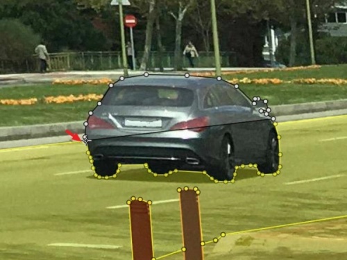
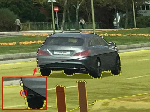
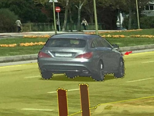
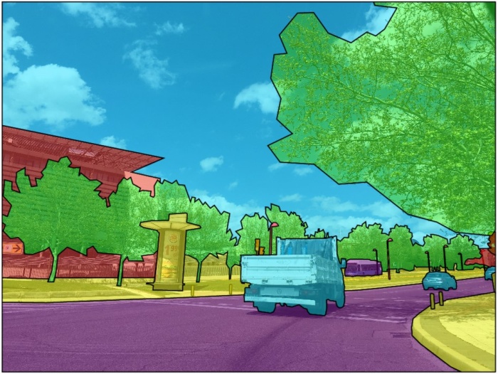
Occlusion is an attribute used if an object is occluded by another object or
isn’t fully visible on the frame. Use Q shortcut to set the property
quickly.
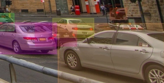
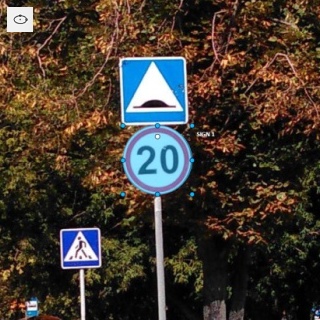
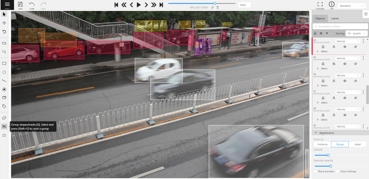
Example: the three cars on the figure below should be labeled as occluded.
If a frame contains too many objects and it is difficult to annotate them
due to many shapes placed mostly in the same place, it makes sense
to lock them. Shapes for locked objects are transparent, and it is easy to
annotate new objects. Besides, you can’t change previously annotated objects
by accident. Shortcut: L.
2 - Single Shape
The CVAT Single Shape annotation mode accelerates the annotation process and enhances workflow efficiency for specific scenarios.
By using this mode you can label objects with a chosen annotation shape and label when an image contains only a single object. By eliminating the necessity to select tools from the sidebar and facilitating quicker navigation between images without the reliance on hotkeys, this feature makes the annotation process significantly faster.
See:
- Single Shape mode annotation interface
- Annotating in Single Shape mode
- Query parameters
- Video tutorial
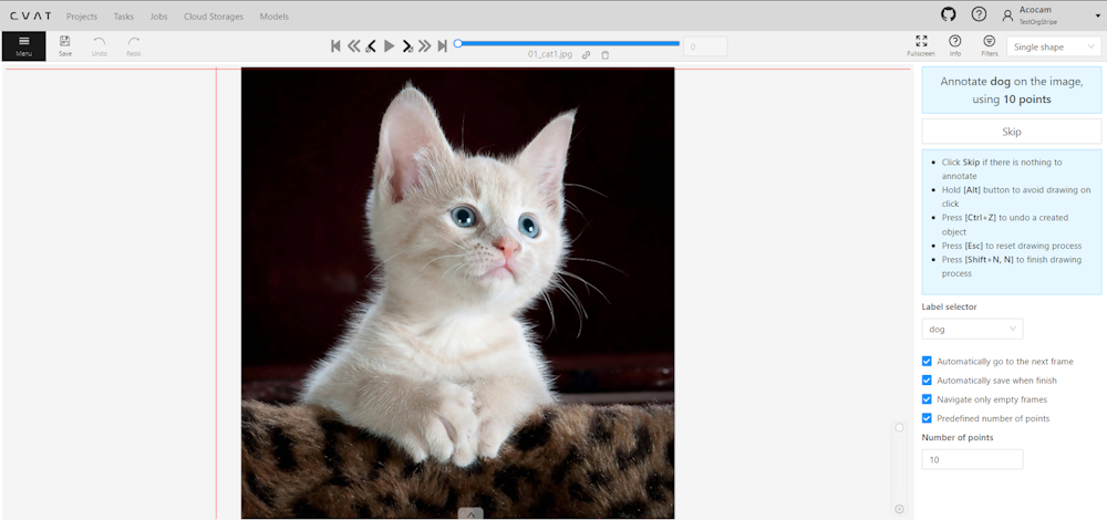
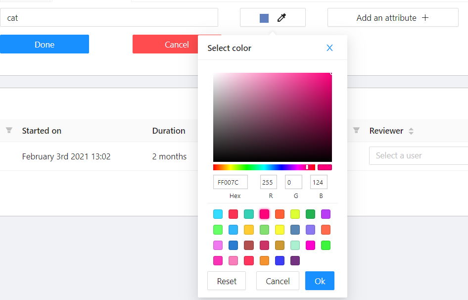
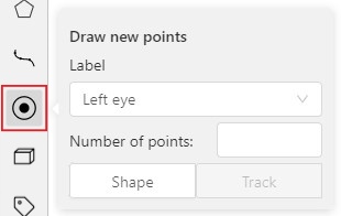
Single Shape mode annotation interface
A set of controls in the interface of the Single Shape annotation mode may vary depending on different settings.
Images below displays the complete interface, featuring all available fields; as mentioned above, certain fields may be absent depending on the scenario.
For instance, when annotating with rectangles, the Number of points field will not appear, and if annotating a single class, the Labels selector will be omitted.
To access Single Shape mode, open the job, navigate to the top right corner, and from the drop-down menu, select Single Shape.
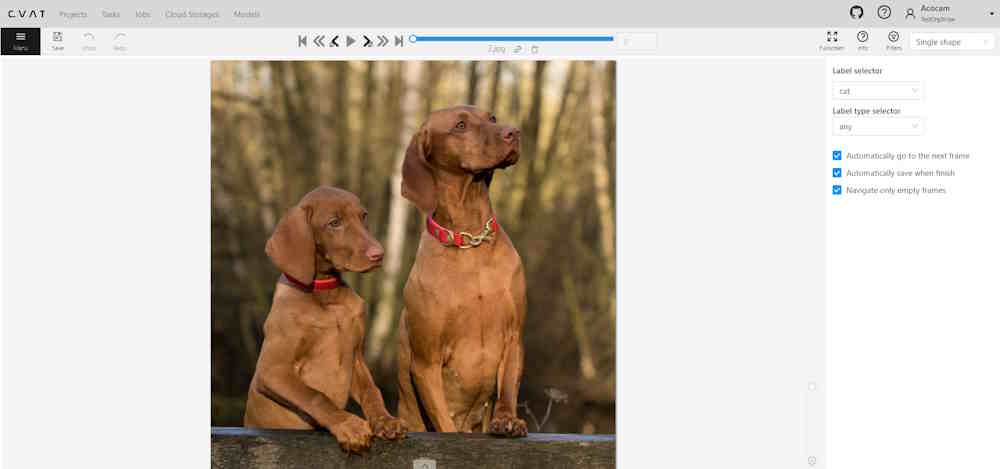
The interface will be different if the shape type was set to Any in the label Constructor:
The Single Shape annotation mode has the following fields:
| Feature | Explanation |
|---|---|
| Prompt for Shape and Label | Displays the selected shape and label for the annotation task, for example: “Annotate cat on the image using rectangle”. |
| Skip Button | Enables moving to the next frame without annotating the current one, particularly useful when the frame does not have anything to be annotated. |
| List of Hints | Offers guidance on using the interface effectively, including: - Click Skip for frames without required annotations. - Hold the Alt button to avoid unintentional drawing (e.g. when you want only move the image). - Use the Ctrl+Z combination to undo the last action if needed. - Use the Esc button to completely reset the current drawing progress. |
| Label selector | Allows for the selection of different labels (cat, or dog in our example) for annotation within the interface. |
| Label type selector | A drop-down list to select type of the label (rectangle, ellipse, etc). Only visible when the type of the shape is Any. |
| Options to Enable or Disable | Provides configurable options to streamline the annotation process, such as: - Automatically go to the next frame. - Automatically save when finish. - Navigate only empty frames. - Predefined number of points - Specific to polyshape annotations, enabling this option auto-completes a shape once a predefined number of points is reached. Otherwise, pressing N is required to finalize the shape. |
| Number of Points | Applicable for polyshape annotations, indicating the number of points to use for image annotation. |
Annotating in Single Shape mode
To annotate in Single Shape mode, follow these steps:
- Open the job and switch to Single Shape mode.
- Annotate the image based on the selected shape. For more information on shapes, see Annotation Tools.
- (Optional) If the image does not contain any objects to annotate, click Skip at the top of the right panel.
- Submit your work.
Query parameters
Also, we introduced additional query parameters, which you may append to the job link, to initialize the annotation process and automate workflow:
| Query Parameter | Possible Values | Explanation |
|---|---|---|
defaultWorkspace |
Workspace identifier (e.g., single_shape, tags, review, attributes) |
Specifies the workspace to be used initially, streamlining the setup for different annotation tasks. |
defaultLabel |
A string representation of a label (label name) | Sets a default label for the annotation session, facilitating consistency across similar tasks. |
defaultPointsCount |
Integer - number of points for polyshapes | Defines a preset number of points for polyshape annotations, optimizing the annotation process. |
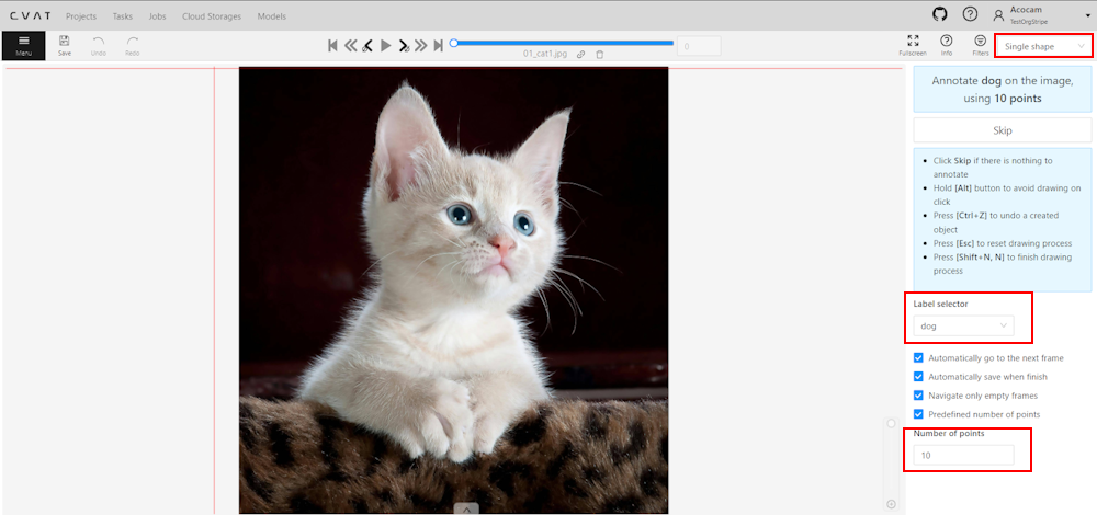
You can combine these parameters to customize the workspace for an annotator, for example:
/tasks/<tid>/jobs/<jid>?defaultWorkspace=single_shape&defaultLabel=dog&defaultPointsCount=10
Will open the following job:
Video tutorial
For a better understanding of how Single Shape mode operates, we recommend watching the following tutorial.
3 - Track mode (advanced)
Basic operations in the mode were described in section track mode (basics).
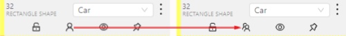
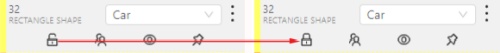
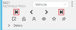
Shapes that were created in the track mode, have extra navigation buttons.
-
These buttons help to jump to the previous/next keyframe.
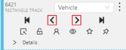
-
The button helps to jump to the initial frame and to the last keyframe.
You can use the Split function to split one track into two tracks:
4 - 3D Object annotation (advanced)
As well as 2D-task objects, 3D-task objects support the ability to change appearance, attributes, properties and have an action menu. Read more in objects sidebar section.
Moving an object
If you hover the cursor over a cuboid and press Shift+N, the cuboid will be cut,
so you can paste it in other place (double-click to paste the cuboid).
Copying
As well as in 2D task you can copy and paste objects by Ctrl+C and Ctrl+V,
but unlike 2D tasks you have to place a copied object in a 3D space (double click to paste).
Image of the projection window
You can copy or save the projection-window image by left-clicking on it and selecting a “save image as” or “copy image”.
Cuboid orientation
The feature enables or disables the display of cuboid orientation arrows in the 3D space. It is controlled by a checkbox located in the appearance block. When enabled, arrows representing the cuboid’s axis orientation (X - red, Y - green, Z - blue) are displayed, providing a visual reference for the cuboid’s alignment within the 3D environment. This feature is useful for understanding the spatial orientation of the cuboid.
Cuboid size input
The size input feature allows users to manually specify the dimensions of a cuboid in the 3D space. This feature is accessible through the objects sidebar - details panel, where you can input precise values for the width, height, and length (X - width, Y - height, Z - length) of the cuboid. By entering these values, the cuboid’s size is adjusted accordingly to its orientation, providing greater control and accuracy when annotating objects in 3D tasks.
5 - Attribute annotation mode (advanced)
Basic operations in the mode were described in section attribute annotation mode (basics).
It is possible to handle lots of objects on the same frame in the mode.
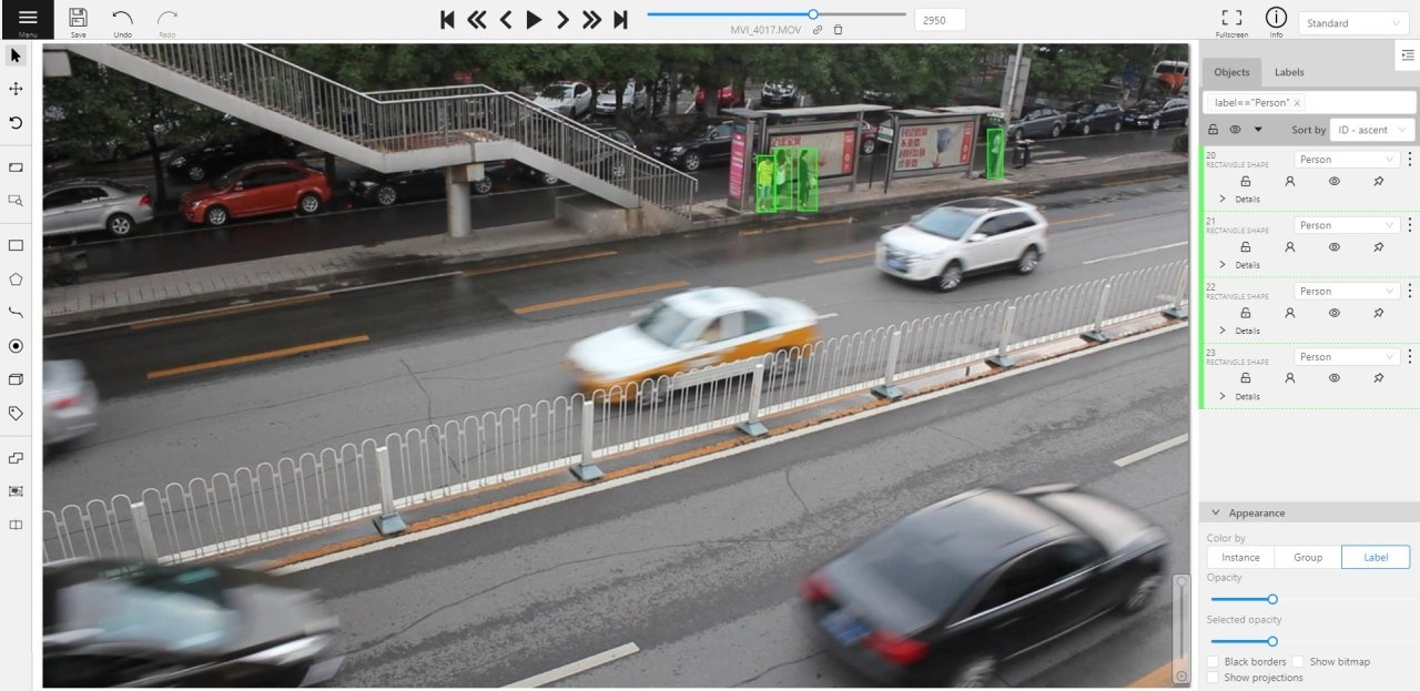
It is more convenient to annotate objects of the same type. In this case you can apply
the appropriate filter. For example, the following filter will
hide all objects except person: label=="Person".
To navigate between objects (person in this case),
use the following buttons switch between objects in the frame on the special panel:
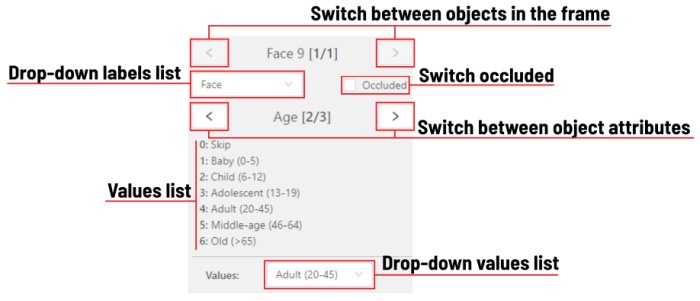
or shortcuts:
Tab— go to the next objectShift+Tab— go to the previous object.
In order to change the zoom level, go to settings (press F3)
in the workspace tab and set the value Attribute annotation mode (AAM) zoom margin in px.
6 - Annotation with rectangles
To learn more about annotation using a rectangle, see the sections:
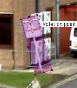
Rotation rectangle
To rotate the rectangle, pull on the rotation point. Rotation is done around the center of the rectangle.
To rotate at a fixed angle (multiple of 15 degrees),
hold shift. In the process of rotation, you can see the angle of rotation.
Annotation with rectangle by 4 points
It is an efficient method of bounding box annotation, proposed here. Before starting, you need to make sure that the drawing method by 4 points is selected.
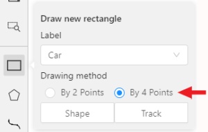
Press Shape or Track for entering drawing mode. Click on four extreme points:
the top, bottom, left- and right-most physical points on the object.
Drawing will be automatically completed right after clicking the fourth point.
Press Esc to cancel editing.
7 - Annotation with polygons
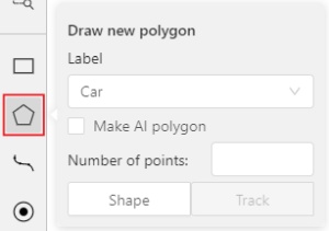
7.1 - Manual drawing
It is used for semantic / instance segmentation.
Before starting, you need to select Polygon on the controls sidebar and choose the correct Label.
- Click
Shapeto enter drawing mode. There are two ways to draw a polygon: either create points by clicking or by dragging the mouse on the screen while holdingShift.
| Clicking points | Holding Shift+Dragging |
|---|---|
 |
 |
- When
Shiftisn’t pressed, you can zoom in/out (when scrolling the mouse wheel) and move (when clicking the mouse wheel and moving the mouse), you can also delete the previous point by right-clicking on it. - You can use the
Selected opacityslider in theObjects sidebarto change the opacity of the polygon. You can read more in the Objects sidebar section. - Press
Nagain or click theDonebutton on the top panel for completing the shape. - After creating the polygon, you can move the points or delete them by right-clicking and selecting
Delete pointor clicking with pressedAltkey in the context menu.
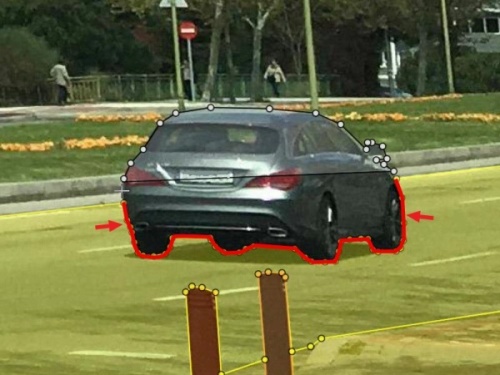
7.2 - Drawing using automatic borders
You can use auto borders when drawing a polygon. Using automatic borders allows you to automatically trace the outline of polygons existing in the annotation.
-
To do this, go to settings -> workspace tab and enable
Automatic Borderingor pressCtrlwhile drawing a polygon.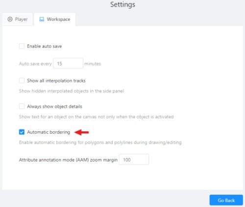
-
Start drawing / editing a polygon.
-
Points of other shapes will be highlighted, which means that the polygon can be attached to them.
-
Define the part of the polygon path that you want to repeat.
-
Click on the first point of the contour part.
-
Then click on any point located on part of the path. The selected point will be highlighted in purple.
-
Click on the last point and the outline to this point will be built automatically.
Besides, you can set a fixed number of points in the Number of points field, then
drawing will be stopped automatically. To enable dragging you should right-click
inside the polygon and choose Switch pinned property.
Below you can see results with opacity and black stroke:
If you need to annotate small objects, increase Image Quality to
95 in Create task dialog for your convenience.
7.3 - Edit polygon
To edit a polygon you have to click on it while holding Shift, it will open the polygon editor.
-
In the editor you can create new points or delete part of a polygon by closing the line on another point.
-
When
Intelligent polygon croppingoption is activated in the settings, CVAT considers two criteria to decide which part of a polygon should be cut off during automatic editing.- The first criteria is a number of cut points.
- The second criteria is a length of a cut curve.
If both criteria recommend to cut the same part, algorithm works automatically, and if not, a user has to make the decision. If you want to choose manually which part of a polygon should be cut off, disable
Intelligent polygon croppingin the settings. In this case after closing the polygon, you can select the part of the polygon you want to leave.
-
You can press
Escto cancel editing.
7.4 - Track mode with polygons
Polygons in the track mode allow you to mark moving objects more accurately other than using a rectangle (Tracking mode (basic); Tracking mode (advanced)).
-
To create a polygon in the track mode, click the
Trackbutton.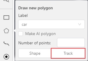
-
Create a polygon the same way as in the case of Annotation with polygons. Press
Nor click theDonebutton on the top panel to complete the polygon. -
Pay attention to the fact that the created polygon has a starting point and a direction, these elements are important for annotation of the following frames.
-
After going a few frames forward press
Shift+N, the old polygon will disappear and you can create a new polygon. The new starting point should match the starting point of the previously created polygon (in this example, the top of the left mirror). The direction must also match (in this example, clockwise). After creating the polygon, pressNand the intermediate frames will be interpolated automatically.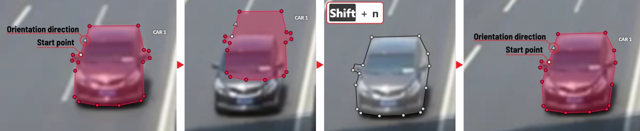
-
If you need to change the starting point, right-click on the desired point and select
Set starting point. To change the direction, right-click on the desired point and select switch orientation.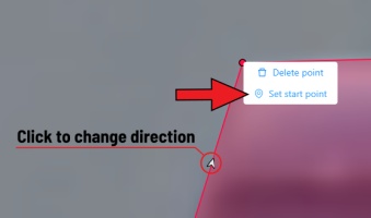
There is no need to redraw the polygon every time using Shift+N,
instead you can simply move the points or edit a part of the polygon by pressing Shift+Click.
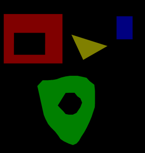
7.5 - Creating masks
Cutting holes in polygons
Currently, CVAT does not support cutting transparent holes in polygons. However, it is possible to generate holes in exported instance and class masks. To do this, one needs to define a background class in the task and draw holes with it as additional shapes above the shapes needed to have holes:
The editor window:
Remember to use z-axis ordering for shapes by [-] and [+, =] keys.
Exported masks:
Notice that it is currently impossible to have a single instance number for internal shapes (they will be merged into the largest one and then covered by “holes”).
Creating masks
There are several formats in CVAT that can be used to export masks:
Segmentation Mask(PASCAL VOC masks)CamVidMOTSICDARCOCO(RLE-encoded instance masks, guide)Datumaro
An example of exported masks (in the Segmentation Mask format):
Important notices:
- Both boxes and polygons are converted into masks
- Grouped objects are considered as a single instance and exported as a single mask (label and attributes are taken from the largest object in the group)
Class colors
All the labels have associated colors, which are used in the generated masks. These colors can be changed in the task label properties:
Label colors are also displayed in the annotation window on the right panel, where you can show or hide specific labels (only the presented labels are displayed):
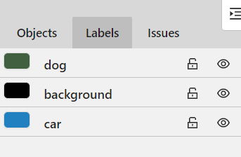
A background class can be:
- A default class, which is implicitly-added, of black color (RGB 0, 0, 0)
backgroundclass with any color (has a priority, name is case-insensitive)- Any class of black color (RGB 0, 0, 0)
To change background color in generated masks (default is black),
change background class color to the desired one.
8 - Annotation with polylines
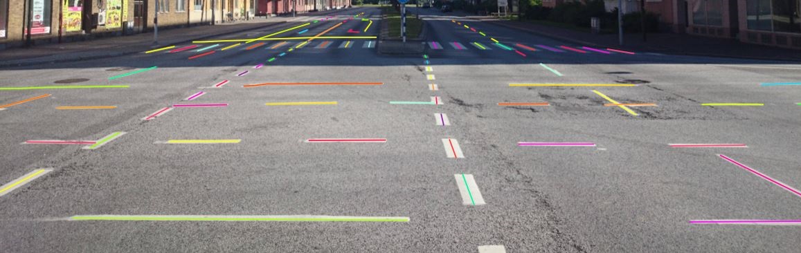
It is used for road markup annotation etc.
Before starting, you need to select the Polyline. You can set a fixed number of points
in the Number of points field, then drawing will be stopped automatically.
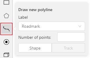
Click Shape to enter drawing mode. There are two ways to draw a polyline —
you either create points by clicking or by dragging a mouse on the screen while holding Shift.
When Shift isn’t pressed, you can zoom in/out (when scrolling the mouse wheel)
and move (when clicking the mouse wheel and moving the mouse), you can delete
previous points by right-clicking on it.
Press N again or click the Done button on the top panel to complete the shape.
You can delete a point by clicking on it with pressed Ctrl or right-clicking on a point
and selecting Delete point. Click with pressed Shift will open a polyline editor.
There you can create new points(by clicking or dragging) or delete part of a polygon closing
the red line on another point. Press Esc to cancel editing.
9 - Annotation with points
9.1 - Points in shape mode
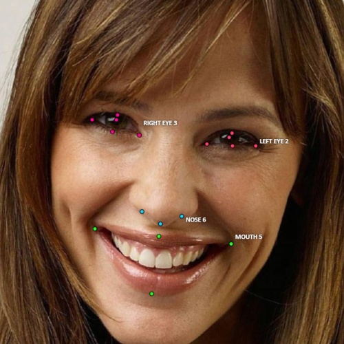
It is used for face, landmarks annotation etc.
Before you start you need to select the Points. If necessary you can set a fixed number of points
in the Number of points field, then drawing will be stopped automatically.
Click Shape to entering the drawing mode. Now you can start annotation of the necessary area.
Points are automatically grouped — all points will be considered linked between each start and finish.
Press N again or click the Done button on the top panel to finish marking the area.
You can delete a point by clicking with pressed Ctrl or right-clicking on a point and selecting Delete point.
Clicking with pressed Shift will open the points shape editor.
There you can add new points into an existing shape. You can zoom in/out (when scrolling the mouse wheel)
and move (when clicking the mouse wheel and moving the mouse) while drawing. You can drag an object after
it has been drawn and change the position of individual points after finishing an object.
9.2 - Linear interpolation with one point
You can use linear interpolation for points to annotate a moving object:
-
Before you start, select the
Points. -
Linear interpolation works only with one point, so you need to set
Number of pointsto 1. -
After that select the
Track.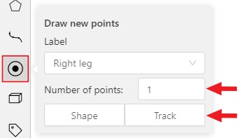
-
Click
Trackto enter the drawing mode left-click to create a point and after that shape will be automatically completed.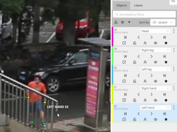
-
Move forward a few frames and move the point to the desired position, this way you will create a keyframe and intermediate frames will be drawn automatically. You can work with this object as with an interpolated track: you can hide it using the
Outside, move around keyframes, etc.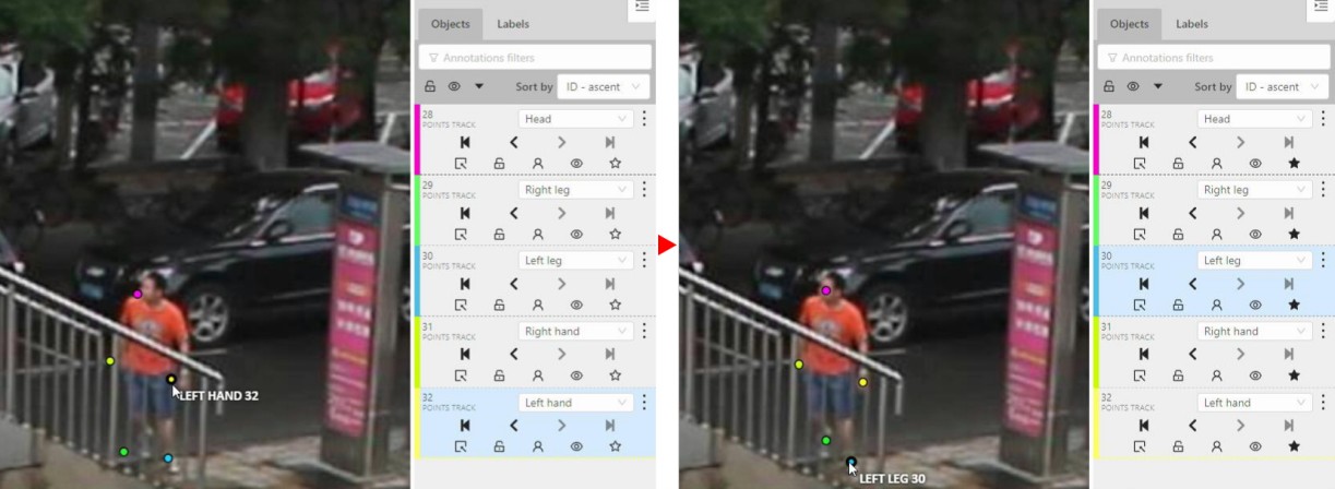
-
This way you’ll get linear interpolation using the
Points.
10 - Annotation with ellipses
It is used for road sign annotation etc.
First of all you need to select the ellipse on the controls sidebar.
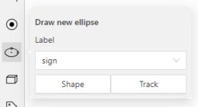
Choose a Label and click Shape or Track to start drawing. An ellipse can be created the same way as
a rectangle,
you need to specify two opposite points,
and the ellipse will be inscribed in an imaginary rectangle. Press N or click the Done button on the top panel
to complete the shape.
You can rotate ellipses using a rotation point in the same way as rectangles.
Annotation with ellipses video tutorial
11 - Annotation with cuboids
It is used to annotate 3 dimensional objects such as cars, boxes, etc… Currently the feature supports one point perspective and has the constraint where the vertical edges are exactly parallel to the sides.
11.1 - Creating the cuboid
Before you start, you have to make sure that Cuboid is selected
and choose a drawing method from rectangle or by 4 points.
Drawing cuboid by 4 points
Choose a drawing method by 4 points and select Shape to enter the drawing mode.
There are many ways to draw a cuboid.
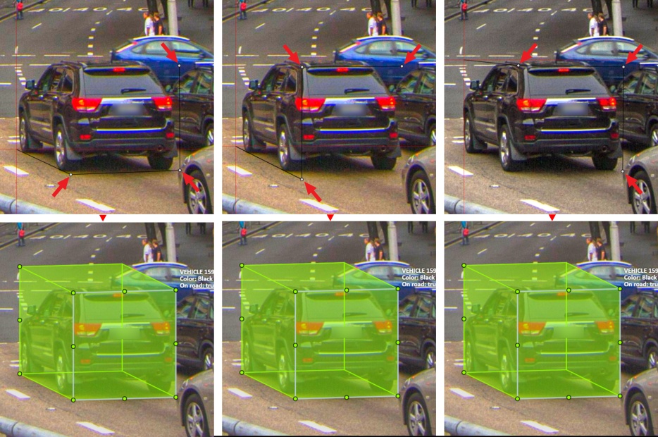
You can draw the cuboid by placing 4 points, after that the drawing will be completed automatically.
The first 3 points determine the plane of the cuboid while the last point determines the depth of that plane.
For the first 3 points, it is recommended to only draw the 2 closest side faces, as well as the top and bottom face.
A few examples:
Drawing cuboid from rectangle
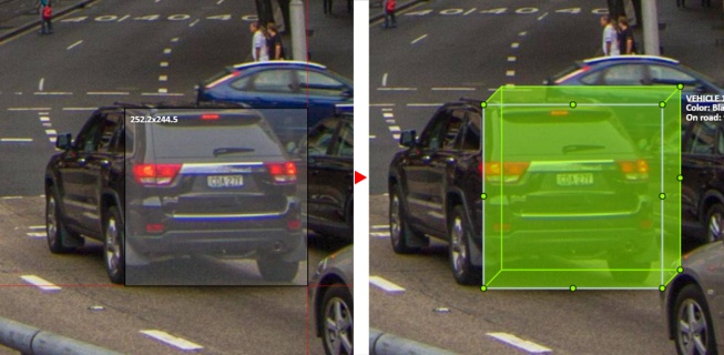
Choose a drawing method from rectangle and select Shape to enter the drawing mode.
When you draw using the rectangle method, you must select the frontal plane of the object using the bounding box.
The depth and perspective of the resulting cuboid can be edited.
Example:
11.2 - Editing the cuboid
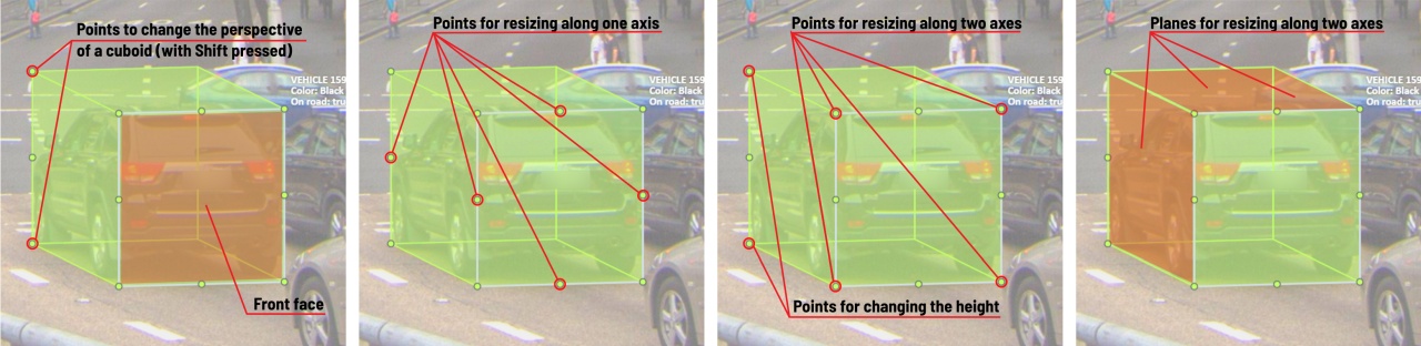
The cuboid can be edited in multiple ways: by dragging points, by dragging certain faces or by dragging planes. First notice that there is a face that is painted with gray lines only, let us call it the front face.
You can move the cuboid by simply dragging the shape behind the front face. The cuboid can be extended by dragging on the point in the middle of the edges. The cuboid can also be extended up and down by dragging the point at the vertices.
To draw with perspective effects it should be assumed that the front face is the closest to the camera.
To begin simply drag the points on the vertices that are not on the gray/front face while holding Shift.
The cuboid can then be edited as usual.
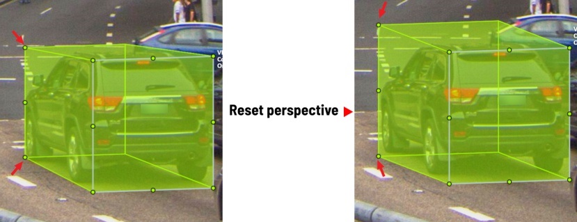
If you wish to reset perspective effects, you may right click on the cuboid,
and select Reset perspective to return to a regular cuboid.
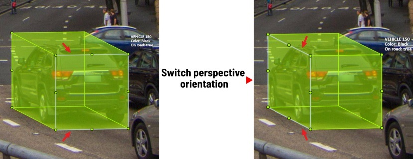
The location of the gray face can be swapped with the adjacent visible side face.
You can do it by right clicking on the cuboid and selecting Switch perspective orientation.
Note that this will also reset the perspective effects.
Certain faces of the cuboid can also be edited, these faces are: the left, right and dorsal faces, relative to the gray face. Simply drag the faces to move them independently from the rest of the cuboid.
You can also use cuboids in track mode, similar to rectangles in track mode (basics and advanced) or Track mode with polygons.
12 - Annotation with skeletons
In this guide, we delve into the efficient process of annotating complex structures through the implementation of Skeleton annotations.
Skeletons serve as annotation templates for annotating complex objects with a consistent structure, such as human pose estimation or facial landmarks.
A Skeleton is composed of numerous points (also referred to as elements), which may be connected by edges. Each point functions as an individual object, possessing unique attributes and properties like color, occlusion, and visibility.
Skeletons can be exported in two formats: CVAT for image and COCO Keypoints.
Note
Skeletons’ labels cannot be imported in a label-less project by importing a dataset. You need to define the labels manually before the import.See:
- Adding Skeleton manually
- Adding Skeleton labels from the model
- Annotation with Skeletons
- Automatic annotation with Skeletons
- Editing skeletons on the canvas
- Editing skeletons on the sidebar
Adding Skeleton manually
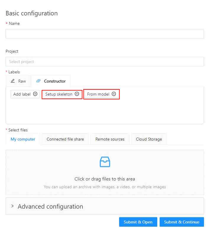
To start annotating using skeletons, you need to set up a Skeleton task in Configurator:
To open Configurator, when creating a task, click on the Setup skeleton button if you want to set up the skeleton manually, or From model if you want to add skeleton labels from a model.
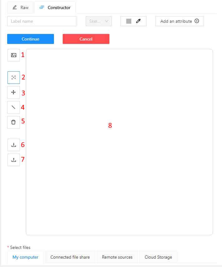
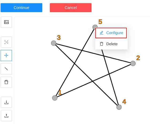
Skeleton Configurator
The skeleton Configurator is a tool to build skeletons for annotation. It has the following fields:
| Number | Name | Description |
|---|---|---|
| 1 | Upload background image | (Optional) Use it to upload a background image, to draw a skeleton on top of it. |
| 2 | Add point | Use it to add Skeleton points to the Drawing area (8). |
| 3 | Click and drag | Use it to move points across the Drawing area (8). |
| 4 | Add edge | Use it to add edge on the Drawing area (8) to connect the points (2). |
| 5 | Remove point | Use it to remove points. Click on Remove point and then on any point (2) on the Drawing area (8) to delete the point. |
| 6 | Download skeleton | Use it to download created skeleton in .SVG format. |
| 7 | Upload skeleton | Use it to upload skeleton in .SVG format. |
| 8 | Drawing area | Use it as a canvas to draw a skeleton. |
Configuring Skeleton points
You can name labels, set attributes, and change the color of each point of the skeleton.
To do this, right-click on the skeleton point and select Configure:
In the opened menu, you can change the point setting. It is similar to adding labels and attributes of the regular task:
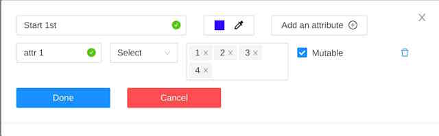
A Skeleton point can only exist within its parent Skeleton.
Note
You cannot change the skeleton configuration for an existing task/project.
You can copy/insert skeleton configuration from the Raw tab of the label configurator.
Adding Skeleton labels manually
To create the Skeleton task, do the following:
- Open Configurator.
- (Optional) Upload background image.
- In the Label name field, enter the name of the label.
- (Optional) Add attribute
Note: you can add attributes exclusively to each point, for more information, see Configuring Skeleton points - Use Add point to add points to the Drawing area.
- Use Add edge to add edges between points.
- Upload files.
- Click:
- Submit & Open to create and open the task.
- Submit & Continue to submit the configuration and start creating a new task.
Adding Skeleton labels from the model
To add points from the model, and annotate do the following:
-
Open Basic configurator.
-
On the Constructor tab, click From model.
-
From the Select a model to pick labels select the
Human pose estimationmodel or others if available. -
Click on the model’s labels, you want to use.
Selected labels will become gray.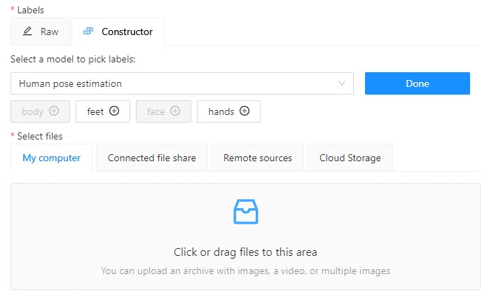
-
(Optional) If you want to adjust labels, within the label, click the Update attributes icon.
The Skeleton configurator will open, where you can configure the skeleton.
Note: Labels cannot be adjusted after the task/project is created. -
Click Done. The labels, that you selected, will appear in the labels window.
-
Upload data.
-
Click:
- Submit & Open to create and open the task.
- Submit & Continue to submit the configuration and start creating a new task.
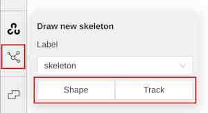
Annotation with Skeletons
To annotate with Skeleton, do the following
-
Open job.
-
On the tools panel select Draw new skeleton.
-
Select Track to annotate with tracking or Shape to annotate without tracking.
-
Draw a skeleton on the image.
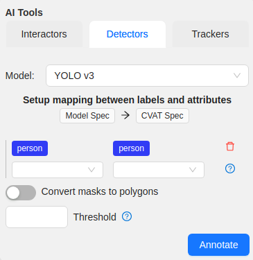
Automatic annotation with Skeletons
To automatically annotate with Skeleton, do the following
-
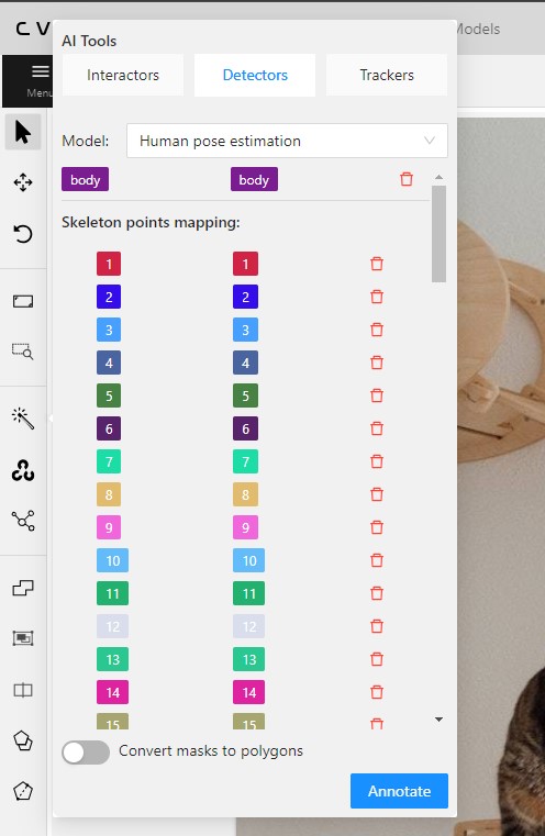
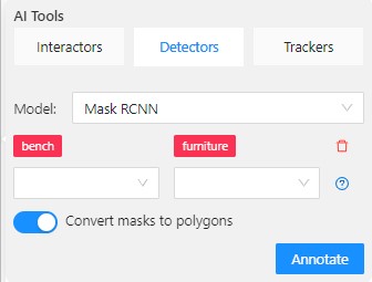
Open the job and on the tools panel select AI Tools > Detectors
-
From the drop-down list select the model. You will see a list of points to match and the name of the skeleton on the top of the list.
-
(Optional) By clicking on the Bin icon, you can remove any mapped item:
- A skeleton together with all points.
- Certain points from two mapped skeletons.
-
Click Annotate.
Editing skeletons on the canvas
A drawn skeleton is encompassed within a bounding box, it allows you to manipulate the skeleton as a regular bounding box, enabling actions such as dragging, resizing, or rotating:
Upon repositioning a point, the bounding box adjusts automatically, without affecting other points:

Additionally, Shortcuts are applicable to both the skeleton as a whole and its elements:
- To use a shortcut to the entire skeleton, hover over the bounding box and push the shortcut keyboard key. This action is applicable for shortcuts like the lock, occluded, pinned, keyframe, and outside for skeleton tracks.
- To use a shortcut to a specific skeleton point, hover over the point and push the shortcut keyboard key. The same list of shortcuts is available, with the addition of outside, which is also applicable to individual skeleton shape elements.
Editing skeletons on the sidebar
In CVAT, the sidebar offers an alternative method for setting up skeleton properties and attributes.
This approach is similar to that used for other object types supported by CVAT, but with a few specific alterations:
An additional collapsible section is provided for users to view a comprehensive list of skeleton parts.
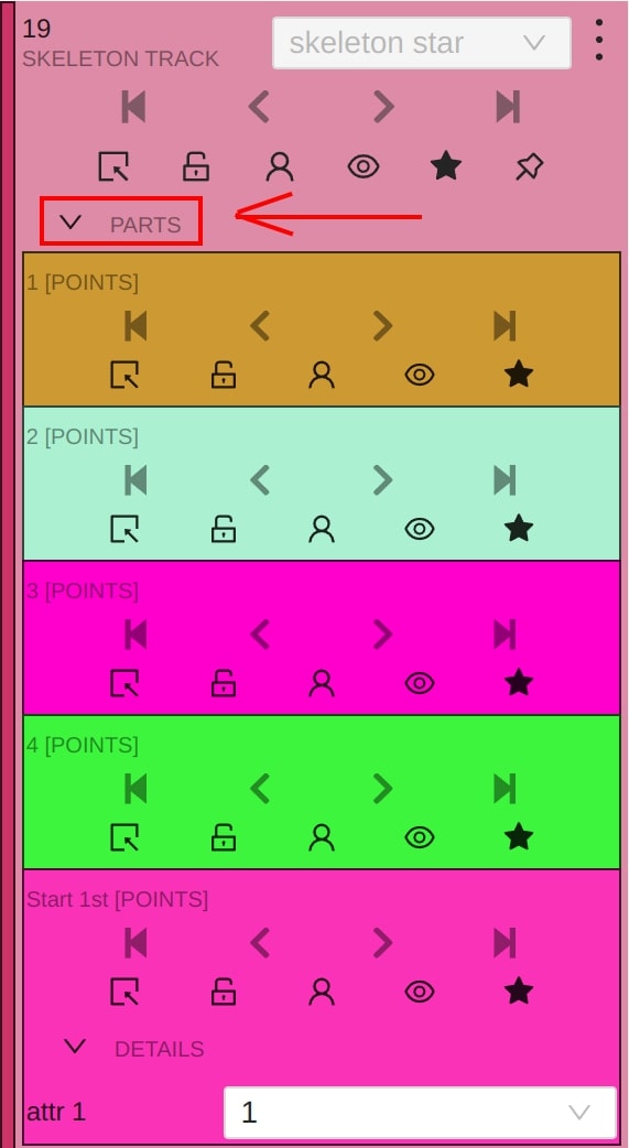
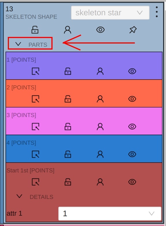
Skeleton points can have properties like Outside, Occluded, and Hidden.
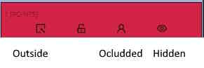
Both Outside and Hidden make a skeleton point invisible.
-
Outside property is part of annotations. Use it when part of the object is out of frame borders.
-
Hidden makes a point hidden only for the annotator’s convenience, this property will not be saved between different sessions.
-
Occluded keeps the point visible on the frame and usually means that the point is still on a frame, just hidden behind another object.
13 - Annotation with brush tool
With a brush tool, you can create masks for disjoint objects, that have multiple parts, such as a house hiding behind trees, a car behind a pedestrian, or a pillar behind a traffic sign. The brush tool has several modes, for example: erase pixels, change brush shapes, and polygon-to-mask mode.
Use brush tool for Semantic (Panoptic) and Instance Image Segmentation tasks.
For more information about segmentation masks in CVAT, see Creating masks.
See:
- Brush tool menu
- Annotation with brush
- Annotation with polygon-to-mask
- Remove underlying pixels
- AI Tools
- Import and export
Brush tool menu
The brush tool menu appears on the top of the screen after you click Shape:

It has the following elements:
| Element | Description | |
|---|---|---|
| Save mask saves the created mask. The saved mask will appear on the object sidebar | ||
 |
Save mask and continue adds a new mask to the object sidebar and allows you to draw a new one immediately. | |
| Brush adds new mask/ new regions to the previously added mask). | ||
 |
Eraser removes part of the mask. | |
 |
Polygon selection tool. Selection will become a mask. | |
 |
Remove polygon selection subtracts part of the polygon selection. | |
 |
Brush size in pixels. Note: Visible only when Brush or Eraser are selected. |
|
 |
Brush shape with two options: circle and square. Note: Visible only when Brush or Eraser are selected. |
|
| Remove underlying pixels. When you are drawing or editing a mask with this tool, pixels on other masks that are located at the same positions as the pixels of the current mask are deleted. |
||
 |
Hide mask. When drawing or editing a mask, you can enable this feature to temporarily hide the mask, allowing you to see the objects underneath more clearly. | |
 |
Label that will be assigned to the newly created mask | |
 |
Move. Click and hold to move the menu bar to the other place on the screen |
Annotation with brush
To annotate with brush, do the following:
-
From the controls sidebar, select Brush
 .
. -
In the Draw new mask menu, select label for your mask, and click Shape.
The Brush tool will be selected by default.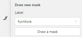
-
With the brush, draw a mask on the object you want to label.
To erase selection, use Eraser
-
After you applied the mask, on the top menu bar click Save mask

to finish the process (or N on the keyboard). -
Added object will appear on the objects sidebar.
To add the next object, repeat steps 1 to 5. All added objects will be visible on the image and the objects sidebar.
To save the job with all added objects, on the top menu, click Save  .
.
Annotation with polygon-to-mask
To annotate with polygon-to-mask, do the following:
-
From the controls sidebar, select Brush
. -
In the Draw new mask menu, select label for your mask, and click Shape.
-
In the brush tool menu, select Polygon
. -
With the Polygon
tool, draw a mask for the object you want to label.
To correct selection, use Remove polygon selection. -
Use Save mask
(or N on the keyboard)
to switch between add/remove polygon tools:
-
After you added the polygon selection, on the top menu bar click Save mask
to finish the process (or N on the keyboard). -
Click Save mask
again (or N on the keyboard).
The added object will appear on the objects sidebar.
To add the next object, repeat steps 1 to 5.
All added objects will be visible on the image and the objects sidebar.
To save the job with all added objects, on the top menu, click Save .
Remove underlying pixels
Use Remove underlying pixels tool when you want to add a mask and simultaneously delete the pixels of
other masks that are located at the same positions. It is a highly useful feature to avoid meticulous drawing edges twice between two different objects.
![]()
AI Tools
You can convert AI tool masks to polygons. To do this, use the following AI tool menu:
- Go to the Detectors tab.
- Switch toggle Masks to polygons to the right.
- Add source and destination labels from the drop-down lists.
- Click Annotate.
Import and export
For export, see Export dataset
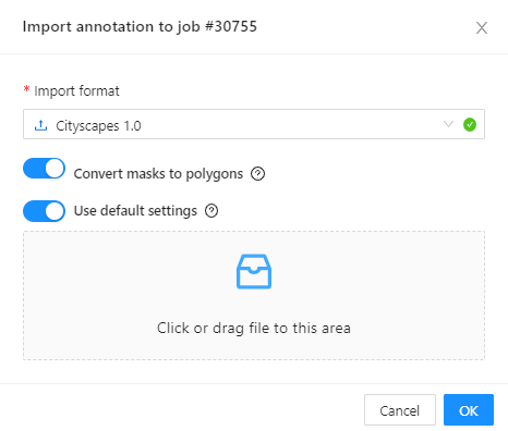
Import follows the general import dataset procedure, with the additional option of converting masks to polygons.
Note
This option is available for formats that work with masks only.To use it, when uploading the dataset, switch the Convert masks to polygon toggle to the right:
14 - Annotation with tags
It is used to annotate frames, tags are not displayed in the workspace.
Before you start, open the drop-down list in the top panel and select Tag annotation.
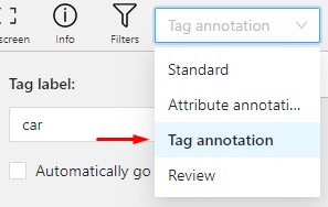
The objects sidebar will be replaced with a special panel for working with tags.
Here you can select a label for a tag and add it by clicking on the Plus button.
You can also customize hotkeys for each label.
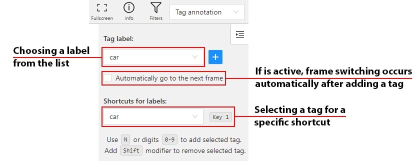
If you need to use only one label for one frame, then enable the Automatically go to the next frame
checkbox, then after you add the tag the frame will automatically switch to the next.
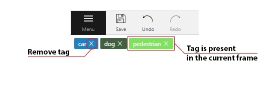
Tags will be shown in the top left corner of the canvas. You can show/hide them in the settings.
15 - AI Tools
Label and annotate your data in semi-automatic and automatic mode with the help of AI and OpenCV tools.
While interpolation is good for annotation of the videos made by the security cameras, AI and OpenCV tools are good for both: videos where the camera is stable and videos, where it moves together with the object, or movements of the object are chaotic.
See:
Interactors
Interactors are a part of AI and OpenCV tools.
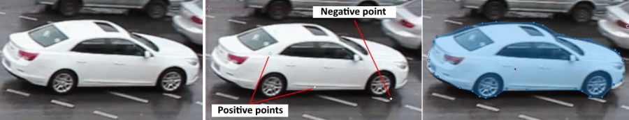
Use interactors to label objects in images by creating a polygon semi-automatically.
When creating a polygon, you can use positive points or negative points (for some models):
- Positive points define the area in which the object is located.
- Negative points define the area in which the object is not located.
AI tools: annotate with interactors
To annotate with interactors, do the following:
- Click Magic wand
 , and go to the Interactors tab.
 - From the Label drop-down, select a label for the polygon.
- From the Interactor drop-down, select a model (see Interactors models).
Click the Question mark to see information about each model: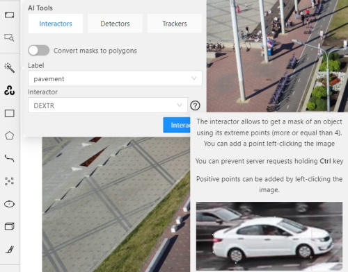
- (Optional) If the model returns masks, and you need to convert masks to polygons, use the Convert masks to polygons toggle.
- Click Interact.
- Use the left click to add positive points and the right click to add negative points.
Number of points you can add depends on the model. - On the top menu, click Done (or Shift+N, N).
AI tools: add extra points
Note
More points improve outline accuracy, but make shape editing harder. Fewer points make shape editing easier, but reduce outline accuracy.Each model has a minimum required number of points for annotation. Once the required number of points is reached, the request is automatically sent to the server. The server processes the request and adds a polygon to the frame.
For a more accurate outline, postpone request to finish adding extra points first:
- Hold down the Ctrl key.
On the top panel, the Block button will turn blue. - Add points to the image.
- Release the Ctrl key, when ready.
In case you used Mask to polygon when the object is finished, you can edit it like a polygon.
You can change the number of points in the polygon with the slider:
AI tools: delete points
To delete a point, do the following:
- With the cursor, hover over the point you want to delete.
- If the point can be deleted, it will enlarge and the cursor will turn into a cross.
- Left-click on the point.
OpenCV: intelligent scissors
To use Intelligent scissors, do the following:
-
On the menu toolbar, click OpenCV
 and wait for the library to load.
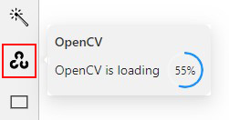
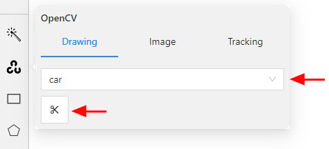
-
Go to the Drawing tab, select the label, and click on the Intelligent scissors button.
-
Add the first point on the boundary of the allocated object.
You will see a line repeating the outline of the object. -
Add the second point, so that the previous point is within the restrictive threshold.
After that a line repeating the object boundary will be automatically created between the points.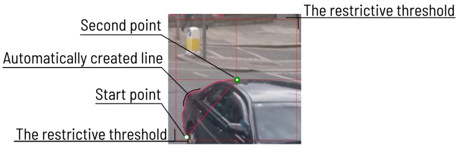
-
To finish placing points, on the top menu click Done (or N on the keyboard).
As a result, a polygon will be created.
You can change the number of points in the polygon with the slider:
To increase or lower the action threshold, hold Ctrl and scroll the mouse wheel.
During the drawing process, you can remove the last point by clicking on it with the left mouse button.
Settings
-
On how to adjust the polygon, see Objects sidebar.
-
For more information about polygons in general, see Annotation with polygons.
Interactors models
| Model | Tool | Description | Example |
|---|---|---|---|
| Segment Anything Model (SAM) | AI Tools | The Segment Anything Model (SAM) produces high quality object masks, and it can be used to generate masks for all objects in an image. It has been trained on a dataset of 11 million images and 1.1 billion masks, and has strong zero-shot performance on a variety of segmentation tasks. For more information, see: |
 |
| Deep extreme cut (DEXTR) |
AI Tool | This is an optimized version of the original model, introduced at the end of 2017. It uses the information about extreme points of an object to get its mask. The mask is then converted to a polygon. For now this is the fastest interactor on the CPU. For more information, see: |
 |
| Inside-Outside-Guidance (IOG) |
AI Tool | The model uses a bounding box and inside/outside points to create a mask. First of all, you need to create a bounding box, wrapping the object. Then you need to use positive and negative points to say the model where is a foreground, and where is a background. Negative points are optional. For more information, see: |
 |
| Intelligent scissors | OpenCV | Intelligent scissors is a CV method of creating a polygon by placing points with the automatic drawing of a line between them. The distance between the adjacent points is limited by the threshold of action, displayed as a red square that is tied to the cursor. For more information, see: |
 |
Detectors
Detectors are a part of AI tools.
Use detectors to automatically identify and locate objects in images or videos.
Labels matching
Each model is trained on a dataset and supports only the dataset’s labels.
For example:
- DL model has the label
car. - Your task (or project) has the label
vehicle.
To annotate, you need to match these two labels to give
DL model a hint, that in this case car = vehicle.
If you have a label that is not on the list of DL labels, you will not be able to match them.
For this reason, supported DL models are suitable only for certain labels.
To check the list of labels for each model, see Detectors models.
Annotate with detectors
To annotate with detectors, do the following:
-
Click Magic wand
, and go to the Detectors tab. -
From the Model drop-down, select model (see Detectors models).
-
From the left drop-down select the DL model label, from the right drop-down select the matching label of your task.
-
(Optional) If the model returns masks, and you need to convert masks to polygons, use the Convert masks to polygons toggle.
-
(Optional) You can specify a Threshold for the model. If not provided, the default value from the model settings will be used.
-
Click Annotate.
This action will automatically annotate one frame. For automatic annotation of multiple frames, see Automatic annotation.
Detectors models
| Model | Description |
|---|---|
| Mask RCNN | The model generates polygons for each instance of an object in the image. For more information, see: |
| Faster RCNN | The model generates bounding boxes for each instance of an object in the image. In this model, RPN and Fast R-CNN are combined into a single network. For more information, see: |
| YOLO v3 | YOLO v3 is a family of object detection architectures and models pre-trained on the COCO dataset. For more information, see: |
| Semantic segmentation for ADAS | This is a segmentation network to classify each pixel into 20 classes. For more information, see: |
| Faster RCNN with Tensorflow | Faster RCNN version with Tensorflow. The model generates bounding boxes for each instance of an object in the image. In this model, RPN and Fast R-CNN are combined into a single network. For more information, see: |
| RetinaNet | Pytorch implementation of RetinaNet object detection. For more information, see: |
| Face Detection | Face detector based on MobileNetV2 as a backbone for indoor and outdoor scenes shot by a front-facing camera. For more information, see: |
Trackers
Trackers are part of AI and OpenCV tools.
Use trackers to identify and label objects in a video or image sequence that are moving or changing over time.
AI tools: annotate with trackers
To annotate with trackers, do the following:
-
Click Magic wand
, and go to the Trackers tab.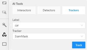
-
From the Label drop-down, select the label for the object.
-
From Tracker drop-down, select tracker.
-
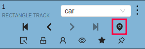
Click Track, and annotate the objects with the bounding box in the first frame.
-
Go to the top menu and click Next (or the F on the keyboard) to move to the next frame.
All annotated objects will be automatically tracked.
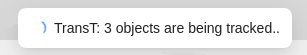
When tracking
-
To enable/disable tracking, use Tracker switcher on the sidebar.
-
Trackable objects have an indication on canvas with a model name.
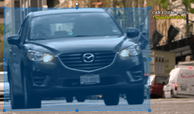
-
You can follow the tracking by the messages appearing at the top.
OpenCV: annotate with trackers
To annotate with trackers, do the following:
-
Create basic rectangle shapes or tracks for tracker initialization
-
On the menu toolbar, click OpenCV
and wait for the library to load. -
From Tracker drop-down, select tracker and Click Track
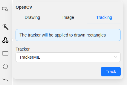
-
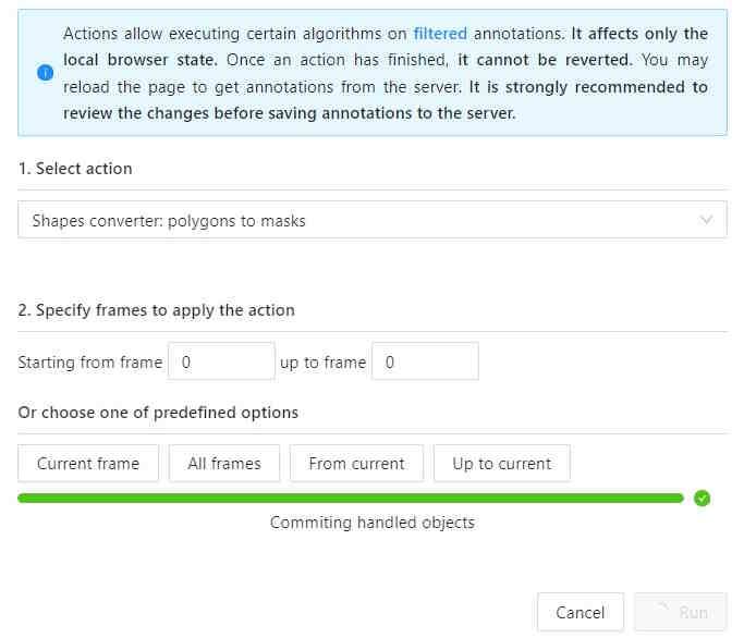
Annotation actions window will pop-up. Setup
Target frameandConvert rectangle shapes to tracksparameters and clickRunNote
Tracking will be applied to all filtered rectangle annotations.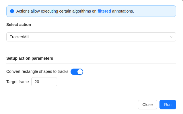
All annotated objects will be automatically tracked up until target frame parameter.
Trackers models
| Model | Tool | Description | Example |
|---|---|---|---|
| TrackerMIL | OpenCV | TrackerMIL model is not bound to labels and can be used for any object. It is a fast client-side model designed to track simple non-overlapping objects. For more information, see: |
|
| SiamMask | AI Tools | Fast online Object Tracking and Segmentation. The trackable object will be tracked automatically if the previous frame was the latest keyframe for the object. For more information, see: |
|
| Transformer Tracking (TransT) | AI Tools | Simple and efficient online tool for object tracking and segmentation. If the previous frame was the latest keyframe for the object, the trackable object will be tracked automatically. This is a modified version of the PyTracking Python framework based on Pytorch For more information, see: |
|
| SAM2 Tracker | AI Agent | Advanced object tracking and segmentation using Meta’s Segment Anything Model 2. Available for CVAT Online and Enterprise via AI agents. Supports polygons and masks with high precision tracking. Requires user-side agent setup with Python 3.10+. For more information, see: |
Example coming soon |
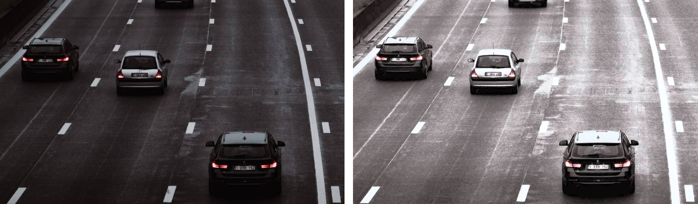
OpenCV: histogram equalization
Histogram equalization improves the contrast by stretching the intensity range.
It increases the global contrast of images when its usable data is represented by close contrast values.
It is useful in images with backgrounds and foregrounds that are bright or dark.
To improve the contrast of the image, do the following:
- In the OpenCV menu, go to the Image tab.
- Click on Histogram equalization button.
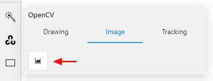
Histogram equalization will improve contrast on current and following frames.
Example of the result:
To disable Histogram equalization, click on the button again.
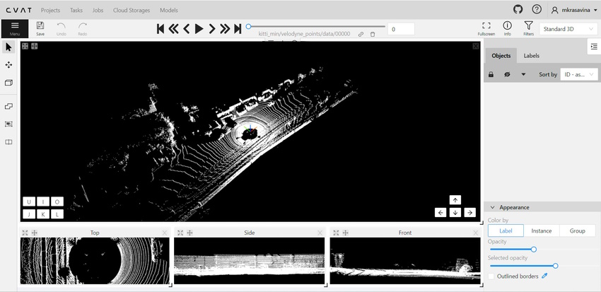
16 - Standard 3D mode (basics)
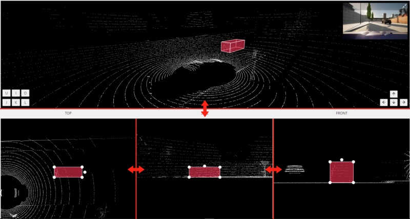
Standard 3d mode - Designed to work with 3D data.
The mode is automatically available if you add PCD or Kitty BIN format data when you create a task
(read more).
You can adjust the size of the projections, to do so, simply drag the boundary between the projections.
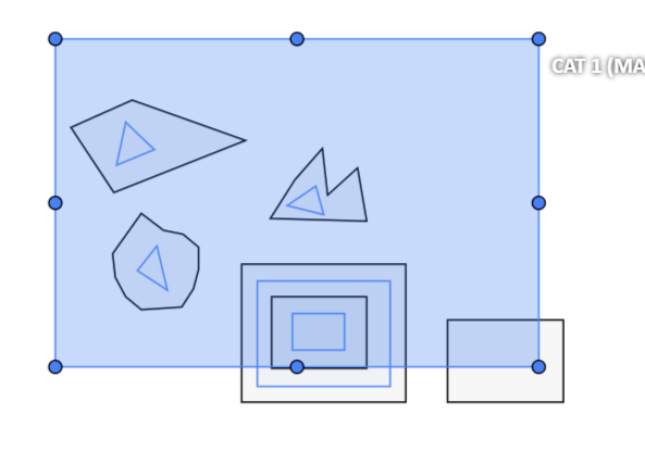
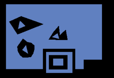
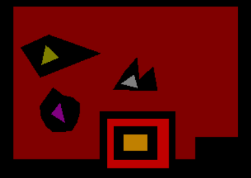
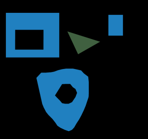
17 - Types of shapes
There are several shapes with which you can annotate your images:
RectangleorBounding boxPolygonPolylinePointsEllipseCuboidCuboid in 3d taskSkeletonTag
And there is what they look like:


Tag - has no shape in the workspace, but is displayed in objects sidebar.
18 - Backup Task and Project
Overview
In CVAT you can backup tasks and projects. This can be used to backup a task or project on your PC or to transfer to another server.
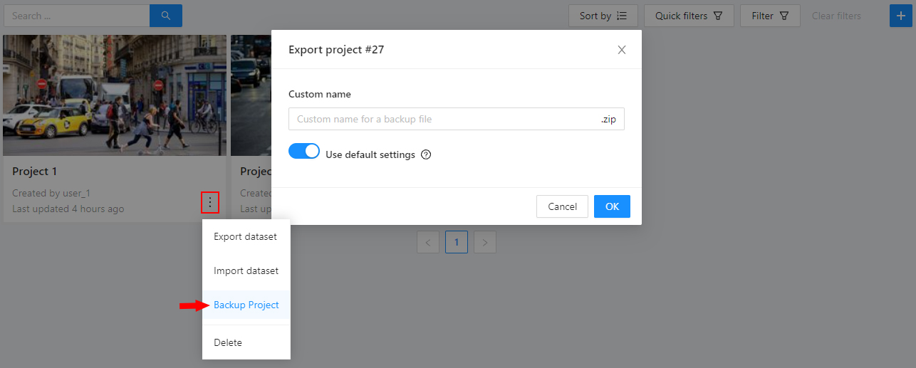
Create backup
To backup a task or project, open the action menu and select Backup Task or Backup Project.
You can backup a project or a task locally on your PC or using an attached cloud storage.
The dialog includes a switch Use lightweight backup whenever possible.
When enabled, CVAT creates a lightweight backup for data that comes from attached cloud storage:
the backup stores task/project meta and annotations and does not copy raw media files.
This reduces backup size and time for cloud-backed data.
The switch has no effect on a tasks, whose data is located on CVAT.
The switch is enabled by default.
(Optional) Specify the name in the Custom name text field for backup, otherwise the file of backup name
will be given by the mask project_<project_name>_backup_<date>_<time>.zip for the projects
and task_<task_name>_backup_<date>_<time>.zip for the tasks.
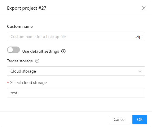
If you want to save a backup to a specific
attached cloud storage,
you should additionally turn off the switch Use default settings, select the Cloud storage value
in the Target storage and select this storage in the list of the attached cloud storages.
Create backup APIs
- endpoints:
/tasks/{id}/backup/projects/{id}/backup
- method:
GET - responses: 202, 201 with zip archive payload
Upload backup APIs
- endpoints:
/api/tasks/backup/api/projects/backup
- method:
POST - Content-Type:
multipart/form-data - responses: 202, 201 with json payload
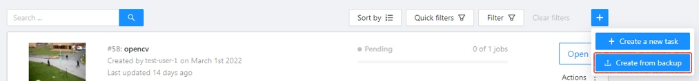
Create from backup
To create a task or project from a backup, go to the tasks or projects page,
click the Create from backup button and select the archive you need.
As a result, you’ll get a task containing data, parameters, and annotations of the previously exported task.
Note: When restoring from a lightweight backup, CVAT creates a task which is not attached to cloud storage. Data cannot be fetched until cloud storage is attached on a Task page.
Backup file structure
As a result, you’ll get a zip archive containing data, task or project and task specification and annotations with the following structure:
    .
    ├── data
    │   └── {user uploaded data}
    ├── task.json
    └── annotations.json
    .
    ├── task_{id}
    │   ├── data
    │   │   └── {user uploaded data}
    │   ├── task.json
    │   └── annotations.json
    └── project.json
19 - Shape mode (basics)
Usage examples:
- Create new annotations for a set of images.
- Add/modify/delete objects for existing annotations.
-
You need to select
Rectangleon the controls sidebar: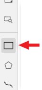
Before you start, select the correct
Label(should be specified by you when creating the task) andDrawing Method(by 2 points or by 4 points):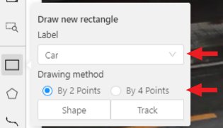
-
Creating a new annotation in
Shape mode:-
Create a separate
Rectangleby selectingShape.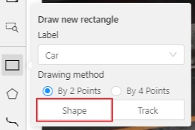
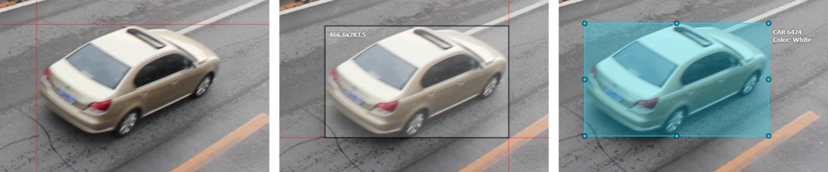
-
Choose the opposite points. Your first rectangle is ready!
-
To learn more about creating a rectangle read here.
-
It is possible to adjust boundaries and location of the rectangle using a mouse. The rectangle’s size is shown in the top right corner, you can check it by selecting any point of the shape. You can also undo your actions using
Ctrl+Zand redo them withShift+Ctrl+ZorCtrl+Y.
-
-
You can see the
Object cardin the objects sidebar or open it by right-clicking on the object. You can change the attributes in the details section. You can perform basic operations or delete an object by selecting on the action menu button.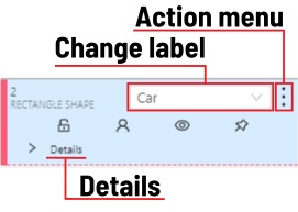
-
The following figure is an example of a fully annotated frame with separate shapes.
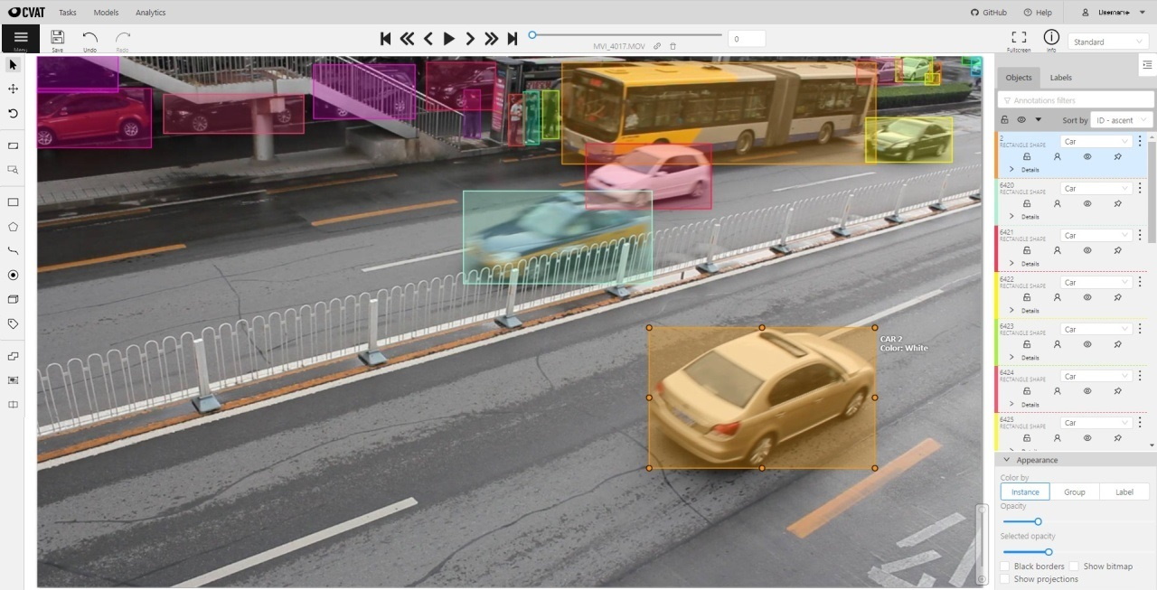
Read more in the section shape mode (advanced).
20 - Frame deleting
Delete frame
You can delete the current frame from a task. This frame will not be presented either in the UI or in the exported annotation. Thus, it is possible to mark corrupted frames that are not subject to annotation.
-
Go to the Job annotation view and click on the Delete frame button (Alt+Del).
Note
When you delete with the shortcut, the frame will be deleted immediately without additional confirmation.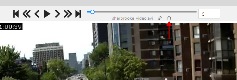
-
After that you will be asked to confirm frame deleting.
Note
all annotations from that frame will be deleted, unsaved annotations will be saved and the frame will be invisible in the annotation view (Until you make it visible in the settings). If there is some overlap in the task and the deleted frame falls within this interval, then this will cause this frame to become unavailable in another job as well. -
When you delete a frame in a job with tracks, you may need to adjust some tracks manually. Common adjustments are:
- Add keyframes at the edges of the deleted interval for the interpolation to look correct;
- Move the keyframe start or end keyframe to the correct side of the deleted interval.
Configure deleted frames visibility and navigation
If you need to enable showing the deleted frames, you can do it in the settings.
-
Go to the settings and chose Player settings.
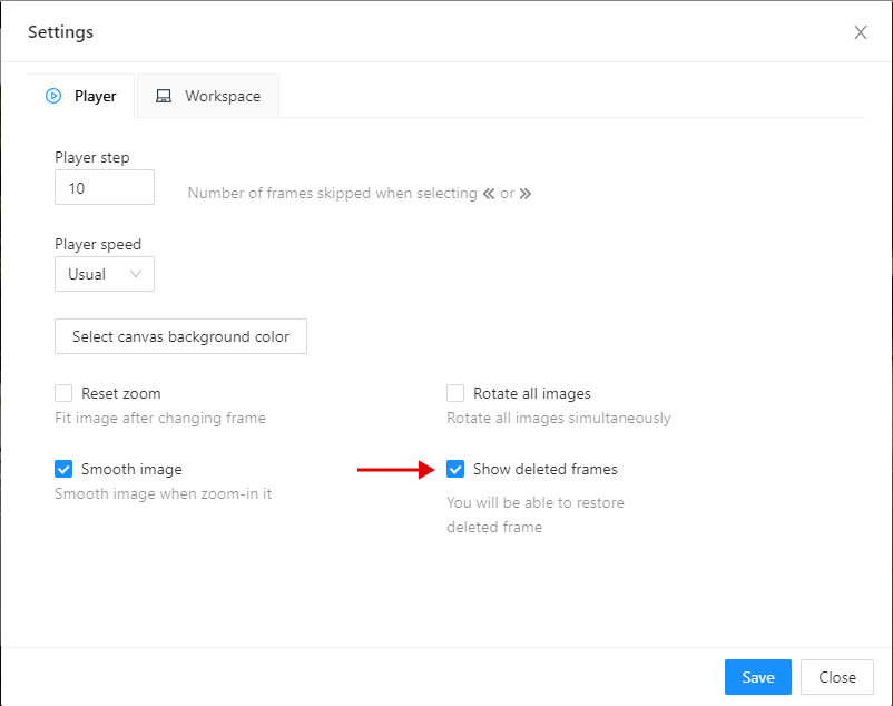
-
Click on the Show deleted frames checkbox. And close the settings dialog.
-
Then you will be able to navigate through deleted frames. But annotation tools will be unavailable. Deleted frames differ in the corresponding overlay.
-
There are ways to navigate through deleted frames without enabling this option:
- Go to the frame via direct navigation methods: navigation slider or frame input field,
- Go to the frame via the direct link, for example:
/api/tasks/{id}/jobs/{id}?frame={frame_id}.
-
Navigation with step will not count deleted frames.
Restore deleted frame
You can also restore deleted frames in the task.
-
Turn on deleted frames visibility, as it was told in the previous part, and go to the deleted frame you want to restore.
-
Click on the Restore icon. The frame will be restored immediately.
21 - Join and slice tools
In CVAT you can modify shapes by either joining multiple shapes into a single label or slicing a single label into several shapes.
This document provides guidance on how to perform these operations effectively.
See:
Joining masks
The Join masks tool (![]() ),
is specifically designed to work with mask annotations.
),
is specifically designed to work with mask annotations.
This tool is useful in scenarios where a single object in an image is annotated with multiple shapes, and there is a need to merge these shapes into a single one.
To join masks, do the following:
- From the Edit block,
select Join masks
 .
. - Click on the canvas area, to select masks that you want to join.
- (Optional) To remove the selection click the mask one more time.
- Click again on Join masks
(J) to execute the join operation.
Upon completion, the selected masks will be joined into a single mask.
Slicing polygons and masks
The Slice mask/polygon (![]() )
is compatible with both mask and polygon annotations.
)
is compatible with both mask and polygon annotations.
This tool is useful in scenarios where multiple objects in an image are annotated with one shape, and there is a need to slice this shape into multiple parts.
Note
The shape can be sliced only in two parts at a time. Use the slice tool several times to split a shape to as many parts as you need.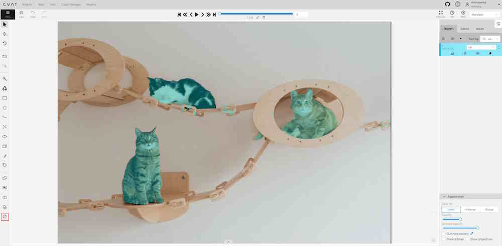
To slice mask or polygon, do the following:
- From the Edit block,
select Slice mask/polygon
 .
. - Click on the shape you intend to slice. A black contour will appear around the selected shape.
- Set an initial point for slicing by clicking on the contour.
- Draw a line across the shape to define the slicing path.
Hold Shift to add points automatically on cursor movement.
Note: The line cannot cross itself.
Note: The line cannot cross the contour more than twice. - (Optional)> Right-click to cancel the latest point.
- Click on the contour (Alt+J) (outside the contour) to finalize the slicing.
22 - Track mode (basics)
Usage examples:
- Create new annotations for a sequence of frames.
- Add/modify/delete objects for existing annotations.
- Edit tracks, merge several rectangles into one track.
-
Like in the
Shape mode, you need to select aRectangleon the sidebar, in the appearing form, select the desiredLabeland theDrawing method.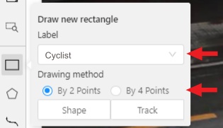
-
Creating a track for an object (look at the selected car as an example):
-
Create a
RectangleinTrack modeby selectingTrack.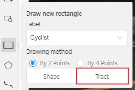
-
In
Track mode, the rectangle will be automatically interpolated on the next frames. -
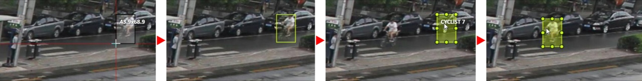
The cyclist starts moving on frame #2270. Let’s mark the frame as a key frame. You can press
Kfor that or select thestarbutton (see the screenshot below).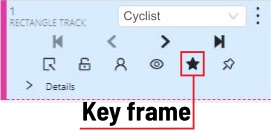
-
If the object starts to change its position, you need to modify the rectangle where it happens. It isn’t necessary to change the rectangle on each frame, simply update several keyframes and the frames between them will be interpolated automatically.
-
Let’s jump 30 frames forward and adjust the boundaries of the object. See an example below:
-
After that the rectangle of the object will be changed automatically on frames 2270 to 2300:
-
-
When the annotated object disappears or becomes too small, you need to finish the track. You have to choose
Outside Property, shortcutO.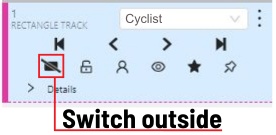
-
If the object isn’t visible on a couple of frames and then appears again, you can use the
Mergefeature to merge several individual tracks into one.
-
Create tracks for moments when the cyclist is visible:
-
Select
Mergebutton or press keyMand select on any rectangle of the first track and on any rectangle of the second track and so on: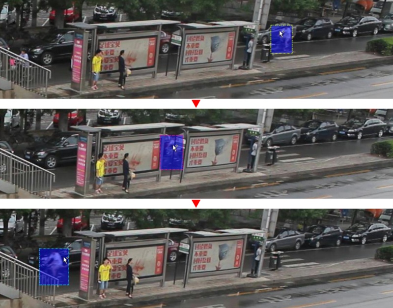
-
Select
Mergebutton or pressMto apply changes. -
The final annotated sequence of frames in
Interpolationmode can look like the clip below:
Read more in the section track mode (advanced).
-
23 - 3D Object annotation
Use the 3D Annotation tool for labeling 3D objects and scenes, such as vehicles, buildings, landscapes, and others.
Check out:
Navigation
The 3D annotation canvas looks like the following:
Note
If you added contextual images to the dataset, the canvas will include them. For more information, consult Contextual imagesFor information on the available tools, consult Controls sidebar.
You can navigate, using the mouse, or navigation keys:
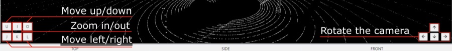
You can also use keyboard shortcuts to navigate:
| Action | Keys |
|---|---|
| Camera rotation | Shift + Arrow (Up, Down, Left, Right) |
| Left/Right | Alt+J/ Alt+L |
| Up/down | Alt+U/ Alt+O |
| Zoom in/ou | Alt+K/ Alt+I |
Annotation with cuboids
There are two options available for 3D annotation:
- Shape: for tasks like object detection.
- Track: uses interpolation to predict the position of objects in subsequent frames. A unique ID will be assigned to each object and maintained throughout the sequence of images.
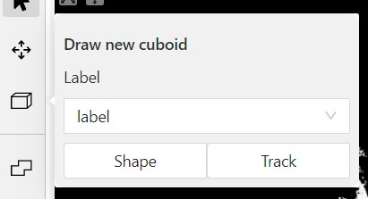
Annotation with shapes
To add a 3D shape:
-
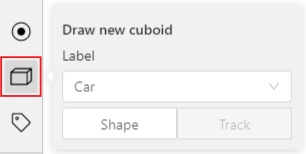
On the objects pane, select Draw new cuboid > select the label from the drop-down list > Shape.
-
The cursor will be followed by a cuboid. Place the cuboid on the 3D scene.
-
Use projections to adjust the cuboid. Click and hold the left mouse button to edit the label shape on the projection.
-
(Optional) Move one of the four points to change the size of the cuboid.
-
(Optional) To rotate the cuboid, select the middle point and then drag the cuboid up/down or to left/right.
Tracking with cuboids
To track with cuboids:
-
On the objects pane, select Draw new cuboid > select the label from the drop-down list > Track.
-
The cursor will be followed by a cuboid. Place the cuboid on the 3D scene.
-
Use projections to adjust the cuboid. Select and hold the left mouse button to edit the label shape on the projection.
-
(Optional) Move one of the four points to change the size of the cuboid.
-
(Optional) To rotate the cuboid, click on the middle point and then drag the cuboid up/down or to left/right.
-
Move several frames forward. You will see the cuboid you’ve added in frame 1. Adjust it, if needed.
-
Repeat to the last frame with the presence of the object you are tracking.
For more information about tracking, consult Track mode.
24 - Attribute annotation mode (basics)
-
In this mode, you can edit attributes with fast navigation between objects and frames using a keyboard. Open the drop-down list in the top panel and select Attribute annotation.
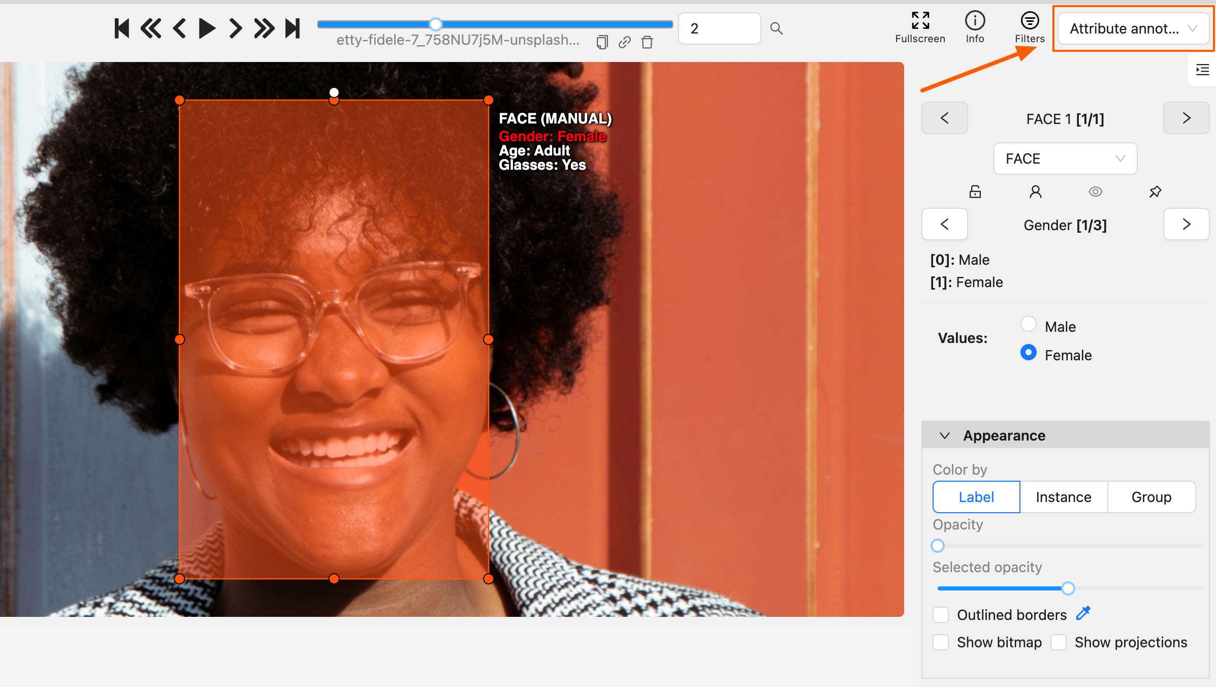
-
In this mode, objects panel change to a special panel:
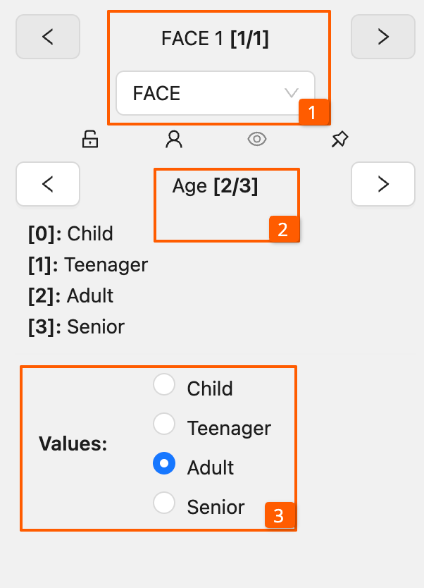
-
The active attribute will be red. In this case, it is
gender. Look at the bottom side panel to see all possible shortcuts for changing the attribute. Press key2on your keyboard to assign a value (female) for the attribute or select from the drop-down list.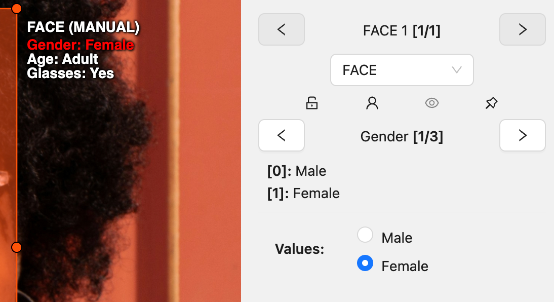
-
Press
Up Arrow/Down Arrowon your keyboard or select the buttons in the UI to go to the next/previous attribute. In this case, after pressingDown Arrowyou will be able to edit theAgeattribute.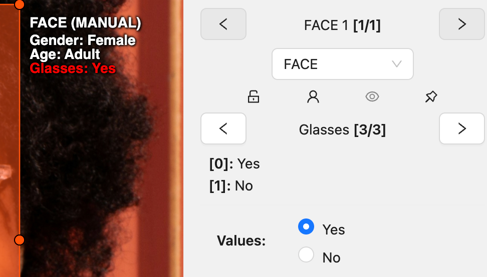
-
Use
Right Arrow/Left Arrowkeys to move to the previous/next image with annotation.
To display all the hot keys available in the attribute annotation mode, press F2.
Learn more in the section
attribute annotation mode (advanced).
25 - Filter
There are some reasons to use the feature:
- When you use a filter, objects that don’t match the filter will be hidden.
- The fast navigation between frames which have an object of interest.
Use the
Left Arrow/Right Arrowkeys for this purpose or customize the UI buttons by right-clicking and selectswitching by filter. If there are no objects which correspond to the filter, you will go to the previous / next frame which contains any annotated objects.
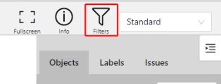
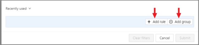
To apply filters you need to click on the button on the top panel.
Create a filter
It will open a window for filter input. Here you will find two buttons: Add rule and Add group.
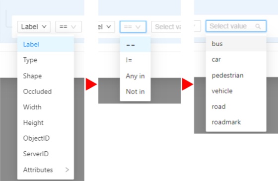
Rules
The Add rule button adds a rule for objects display. A rule may use the following properties:
Supported properties for annotation
| Properties | Supported values | Description |
|---|---|---|
Label |
all the label names that are in the task | label name |
Type |
shape, track or tag | type of object |
Shape |
all shape types | type of shape |
Occluded |
true or false | occluded (read more) |
Width |
number of px or field | shape width |
Height |
number of px or field | shape height |
ServerID |
number or field | ID of the object on the server (You can find out by forming a link to the object through the Action menu) |
ObjectID |
number or field | ID of the object in your client (indicated on the objects sidebar) |
Attributes |
some other fields including attributes with a similar type or a specific attribute value |
any fields specified by a label |
- Supported properties for projects list
- Supported properties for tasks list
- Supported properties for jobs list
- Supported properties for cloud storages list
Supported operators for properties
== - Equally; != - Not equal; > - More; >= - More or equal; < - Less; <= - Less or equal;
Any in; Not in - these operators allow you to set multiple values in one rule;
Is empty; is not empty – these operators don’t require to input a value.
Between; Not between – these operators allow you to choose a range between two values.
Like - this operator indicate that the property must contain a value.
Starts with; Ends with - filter by beginning or end.
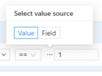
Some properties support two types of values that you can choose:
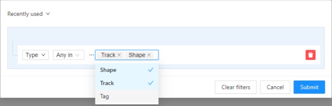
You can add multiple rules, to do so click the add rule button and set another rule.
Once you’ve set a new rule, you’ll be able to choose which operator they will be connected by: And or Or.
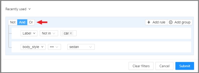
All subsequent rules will be joined by the chosen operator.
Click Submit to apply the filter or if you want multiple rules to be connected by different operators, use groups.
Groups
To add a group, click the Add group button. Inside the group you can create rules or groups.
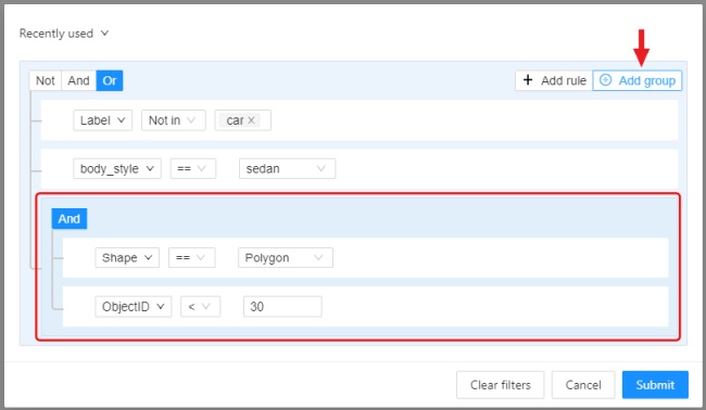
If there is more than one rule in the group, they can be connected by And or Or operators.
The rule group will work as well as a separate rule outside the group and will be joined by an
operator outside the group.
You can create groups within other groups, to do so you need to click the add group button within the group.
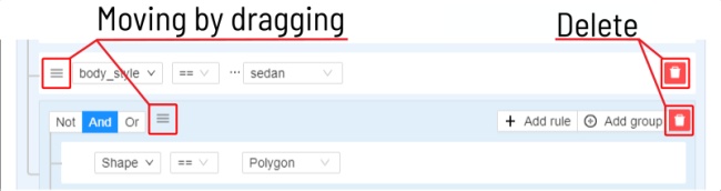
You can move rules and groups. To move the rule or group, drag it by the button.
To remove the rule or group, click on the Delete button.
If you activate the Not button, objects that don’t match the group will be filtered out.
Click Submit to apply the filter.
The Cancel button undoes the filter. The Clear filter button removes the filter.
Once applied filter automatically appears in Recent used list. Maximum length of the list is 10.
Sort and filter lists
On the projects, task list on the project page, tasks, jobs, and cloud storage pages, you can use sorting and filters.
Note
The applied filter and sorting will be displayed in the URL of your browser, Thus, you can share the page with sorting and filter applied.Sort by
You can sort by the following parameters:
- Jobs list: ID, assignee, updated date, stage, state, task ID, project ID, task name, project name.
- Tasks list or tasks list on project page: ID, owner, status, assignee, updated date, subset, mode, dimension, project ID, name, project name.
- Projects list: ID, assignee, owner, status, name, updated date.
- Cloud storages list: ID, provider type, updated date, display name, resource, credentials, owner, description.
To apply sorting, drag the parameter to the top area above the horizontal bar. The parameters below the horizontal line will not be applied. By moving the parameters you can change the priority, first of all sorting will occur according to the parameters that are above.
Pressing the Sort button switches Ascending sort/Descending sort.
Quick filters
Quick Filters contain several frequently used filters:
Assigned to me- show only those projects, tasks or jobs that are assigned to you.Owned by me- show only those projects or tasks that are owned by you.Not completed- show only those projects, tasks or jobs that have a status other than completed.AWS storages- show only AWS cloud storagesAzure storages- show only Azure cloud storagesGoogle cloud storages- show only Google cloud storages
Date and time selection
When creating a Last updated rule, you can select the date and time by using the selection window.
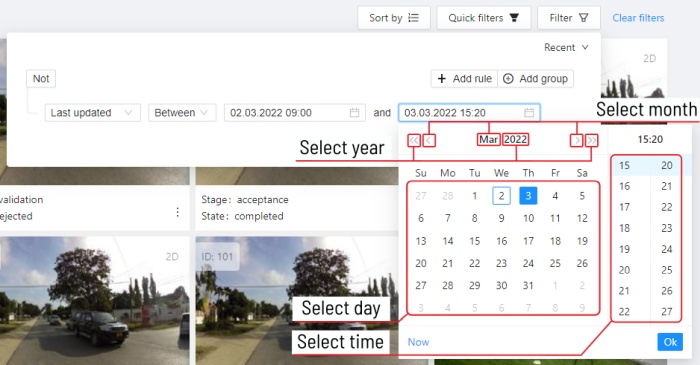
You can select the year and month using the arrows or by clicking on the year and month.
To select a day, click on it in the calendar,
To select the time, you can select the hours and minutes using the scrolling list.
Or you can select the current date and time by clicking the Now button.
To apply, click Ok.
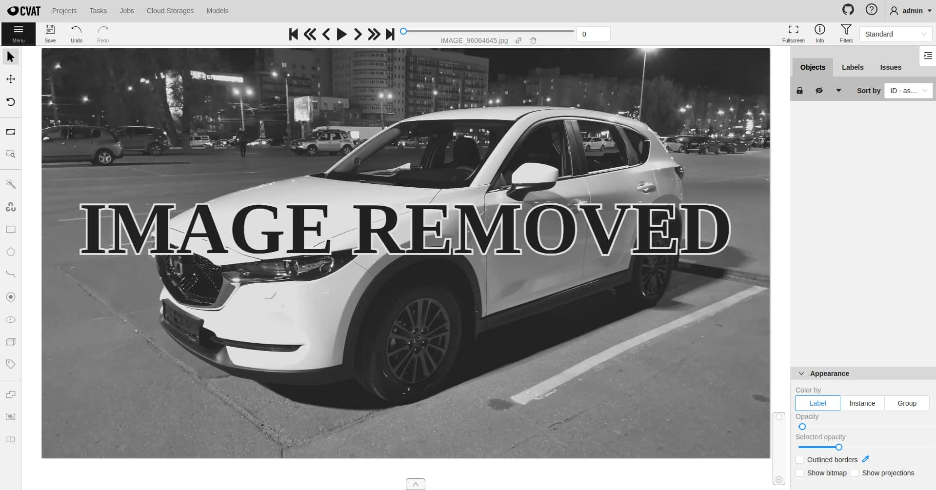
26 - Contextual images
Contextual images (or related images) are additional images that provide context or additional information related to the primary image.
Use them to add extra contextual about the object to improve the accuracy of annotation.
Contextual images are available for 2D and 3D tasks.
See:
Folder structure
To add contextual images to the task, you need to organize the images folder into one of the supported file layouts. A task with contextual images can be created both from an archive or from raw files.
Example for 2D tasks:
- In the folder with the images for annotation, create a folder:
related_images. - Add to the
related_imagesa subfolder with the same name as the primary image to which it should be linked. - Place the contextual image(s) within the subfolder created in step 2.
- Add folder to the archive.
- Create task.
Supported file layouts for 2D and 3D tasks:
root_directory/
  image_1_to_be_annotated.jpg
  image_2_to_be_annotated.jpg
  related_images/
    image_1_to_be_annotated_jpg/
      context_image_for_image_1.jpg
    image_2_to_be_annotated_jpg/
      context_image_for_image_2.jpg
    subdirectory_example/
      image_3_to_be_annotated.jpg
        related_images/
        image_3_to_be_annotated_jpg/
            context_image_for_image_3.jpg
Point clouds and related images are put into the same directory. Related files must have the same names as the corresponding point clouds. This format is limited by only 1 related image per point cloud.
root_directory/
  pointcloud1.pcd
  pointcloud1.jpg
  pointcloud2.pcd
  pointcloud2.png
  ...
Each point cloud is put into a separate directory with matching file name. Related images are put next to the corresponding point cloud, the file names and extensions can be arbitrary.
root_directory/
  pointcloud1/
    pointcloud1.pcd
    pointcloud1_ri1.png
    pointcloud1_ri2.jpg
    ...
  pointcloud2/
    pointcloud2.pcd
    pointcloud2_ri1.bmp
Context images are placed in the image_00/, image_01/, image_N/ (N is any number)
directories. Their file names must correspond to the point cloud files in the data/ directory.
image_00/
  data/
    0000000000.png
    0000000001.png
    0000000002.png
    0000000003.png
image_01/
  data/
    0000000000.png
    0000000001.png
    0000000002.png
    0000000003.png
image_N/
  data/
    0000000000.png
    0000000001.png
    0000000002.png
    0000000003.png
velodyne_points/
  data/
    0000000000.bin
    0000000001.bin
    0000000002.bin
    0000000003.bin
root_directory/
  pointcloud/
    pointcloud1.pcd
    pointcloud2.pcd
  related_images/
    pointcloud1_pcd/
      context_image_for_pointclud1.jpg
    pointcloud2_pcd/
      context_image_for_pointcloud2.jpg
For more general information about 3D data formats, see 3D data formats.
Contextual images
The maximum amount of contextual images is twelve.
By default they will be positioned on the right side of the main image.
Note
By default, only three contextual images will be visible.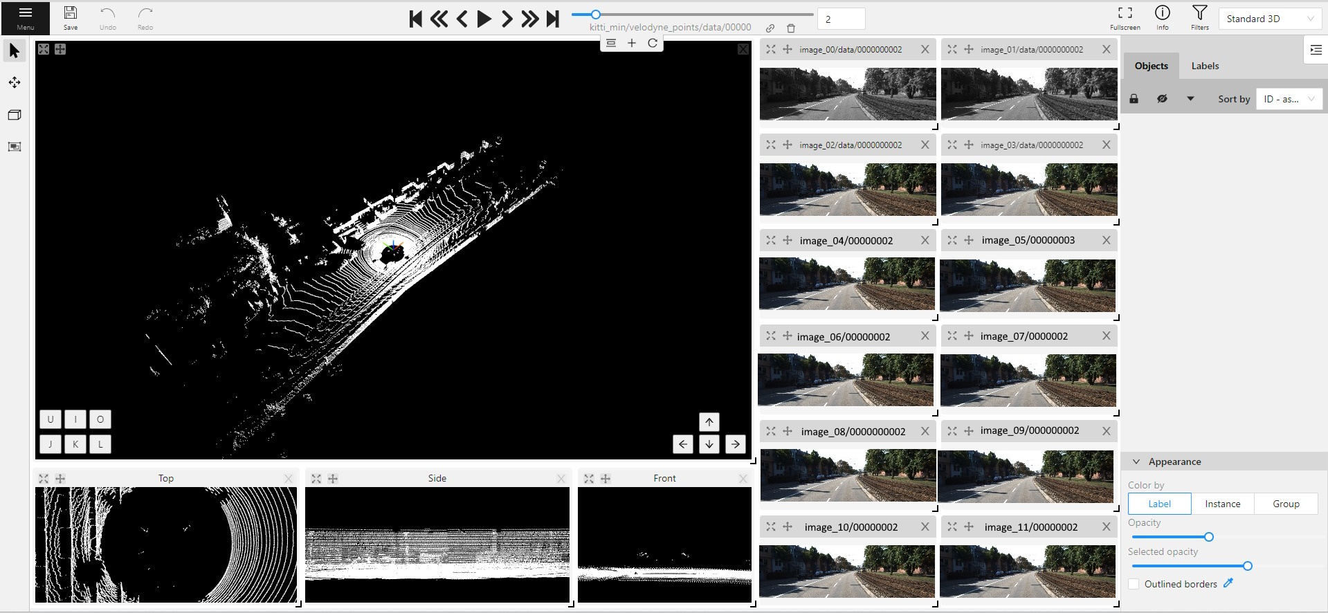
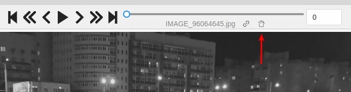
When you add contextual images to the set, small toolbar will appear on the top of the screen, with the following elements:
| Element | Description |
|---|---|
 |
Fit views. Click to restore the layout to its original appearance. If you’ve expanded any images in the layout, they will returned to their original size. This won’t affect the number of context images on the screen. |
 |
Add new image. Click to add context image to the layout. |
 |
Reload layout. Click to reload layout to the default view. Note, that this action can change the number of context images resetting them back to three. |
Each context image has the following elements:
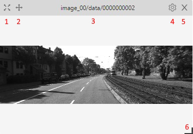
| Element | Description |
|---|---|
| 1 | Full screen. Click to expand the contextual image in to the full screen mode. Click again to revert contextual image to windowed mode. |
| 2 | Move contextual image. Hold and move contextual image to the other place on the screen.
|
| 3 | Name. Unique contextual image name |
| 4 | Select contextual image. Click to open a horizontal listview of all available contextual images. Click on one to select. |
| 5 | Close. Click to remove image from contextual images menu. |
| 6 | Extend Hold and pull to extend the image. |
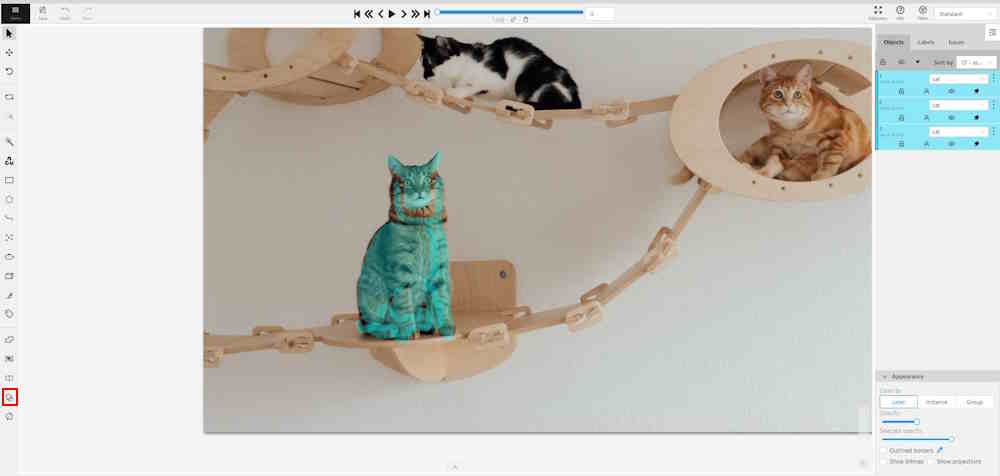
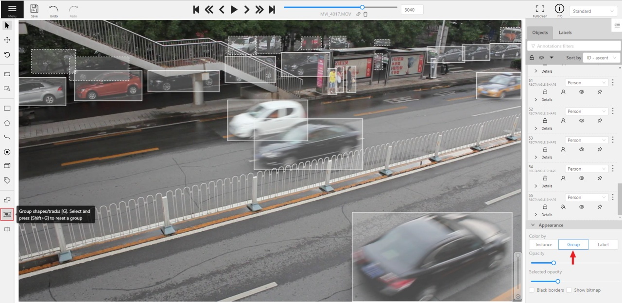
27 - Shape grouping
This feature allows us to group several shapes.
You may use the Group Shapes button or shortcuts:
G— start selection / end selection in group modeEsc— close group modeShift+G— reset group for selected shapes
You may select shapes clicking on them or selecting an area.
Grouped shapes will have group_id filed in dumped annotation.
Also you may switch color distribution from an instance (default) to a group.
You have to switch Color By Group checkbox for that.
Shapes that don’t have group_id, will be highlighted in white.
Shapes grouping video tutorial
28 - Dataset Manifest
Overview
When we create a new task in CVAT, we need to specify where to get the input data from. CVAT allows to use different data sources, including local file uploads, a mounted file share on the server, cloud storages and remote URLs. In some cases CVAT needs to have extra information about the input data. This information can be provided in Dataset manifest files. They are mainly used when working with cloud storages to reduce the amount of network traffic used and speed up the task creation process. However, they can also be used in other cases, which will be explained below.
A dataset manifest file is a text file in the JSONL format. These files can be created automatically with the special command-line tool, or manually, following the manifest file format specification.
How and when to use manifest files
Manifest files can be used in the following cases:
- A video file or a set of images is used as the data source and the caching mode is enabled. Read more
- The data is located in a cloud storage. Read more
- The
predefinedfile sorting method is specified. Read more
The predefined sorting method
Independently of the file source being used, when the predefined
sorting method is selected in the task configuration, the source files will be
ordered according to the .jsonl manifest file, if it is found in the input list of files.
If a manifest is not found, the order provided in the input file list is used.
For image archives (e.g. .zip), a manifest file (*.jsonl) is required when using
the predefined file ordering. A manifest file must be provided next to the archive
in the input list of files, it must not be inside the archive.
If there are multiple manifest files in the input file list, an error will be raised.
How to generate manifest files
CVAT provides a dedicated Python tool to generate manifest files. The source code can be found here.
Using the tool is the recommended way to create manifest files for you data. The data must be available locally to the tool to generate manifest.
Usage
usage: create.py [-h] [--force] [--output-dir .] source

positional arguments:
  source                Source paths

optional arguments:
  -h, --help            show this help message and exit
  --force               Use this flag to prepare the manifest file for video data
                        if by default the video does not meet the requirements
                        and a manifest file is not prepared
  --output-dir OUTPUT_DIR
                        Directory where the manifest file will be saved
Use the script from a Docker image
This is the recommended way to use the tool.
The script can be used from the cvat/server image:
docker run -it --rm -u "$(id -u)":"$(id -g)" \
  -v "${PWD}":"/local" \
  --entrypoint python3 \
  cvat/server \
  utils/dataset_manifest/create.py --output-dir /local /local/<path/to/sources>
Make sure to adapt the command to your file locations.
Use the script directly
Ubuntu 20.04
Install dependencies:
# General
sudo apt-get update && sudo apt-get --no-install-recommends install -y \
    python3-dev python3-pip python3-venv pkg-config
# Library components
sudo apt-get install --no-install-recommends -y \
    libavformat-dev libavcodec-dev libavdevice-dev \
    libavutil-dev libswscale-dev libswresample-dev libavfilter-dev
Create an environment and install the necessary python modules:
python3 -m venv .env
. .env/bin/activate
pip install -U pip
pip install -r utils/dataset_manifest/requirements.in
Note
Please note that if used with video this way, the results may be different from what would the server decode. It is related to the ffmpeg library version. For this reason, using the Docker-based version of the tool is recommended.Examples
Create a dataset manifest in the current directory with video which contains enough keyframes:
python utils/dataset_manifest/create.py ~/Documents/video.mp4
Create a dataset manifest with video which does not contain enough keyframes:
python utils/dataset_manifest/create.py --force --output-dir ~/Documents ~/Documents/video.mp4
Create a dataset manifest with images:
python utils/dataset_manifest/create.py --output-dir ~/Documents ~/Documents/images/
Create a dataset manifest with pattern (may be used *, ?, []):
python utils/dataset_manifest/create.py --output-dir ~/Documents "/home/${USER}/Documents/**/image*.jpeg"
Create a dataset manifest using Docker image:
docker run -it --rm -u "$(id -u)":"$(id -g)" \
  -v ~/Documents/data/:${HOME}/manifest/:rw \
  --entrypoint '/usr/bin/bash' \
  cvat/server \
  utils/dataset_manifest/create.py --output-dir ~/manifest/ ~/manifest/images/
File format
The dataset manifest files are text files in JSONL format. These files have 2 sub-formats: for video and for images and 3d data.
Note
Each top-level entry enclosed in curly braces must use 1 string, no empty strings is allowed. The formatting in the descriptions below is only for demonstration.Dataset manifest for video
The file describes a single video.
pts - time at which the frame should be shown to the user
checksum - md5 hash sum for the specific image/frame decoded
{ "version": <string, version id> }
{ "type": "video" }
{ "properties": {
  "name": <string, filename>,
  "resolution": [<int, width>, <int, height>],
  "length": <int, frame count>
}}
{
  "number": <int, frame number>,
  "pts": <int, frame pts>,
  "checksum": <string, md5 frame hash>
} (repeatable)
Dataset manifest for images and other data types
The file describes an ordered set of images and 3d point clouds.
name - file basename and leading directories from the dataset root
checksum - md5 hash sum for the specific image/frame decoded
{ "version": <string, version id> }
{ "type": "images" }
{
  "name": <string, image filename>,
  "extension": <string, . + file extension>,
  "width": <int, width>,
  "height": <int, height>,
  "meta": <dict, optional>,
  "checksum": <string, md5 hash, optional>
} (repeatable)
Example files
Manifest for a video
{"version":"1.0"}
{"type":"video"}
{"properties":{"name":"video.mp4","resolution":[1280,720],"length":778}}
{"number":0,"pts":0,"checksum":"17bb40d76887b56fe8213c6fded3d540"}
{"number":135,"pts":486000,"checksum":"9da9b4d42c1206d71bf17a7070a05847"}
{"number":270,"pts":972000,"checksum":"a1c3a61814f9b58b00a795fa18bb6d3e"}
{"number":405,"pts":1458000,"checksum":"18c0803b3cc1aa62ac75b112439d2b62"}
{"number":540,"pts":1944000,"checksum":"4551ecea0f80e95a6c32c32e70cac59e"}
{"number":675,"pts":2430000,"checksum":"0e72faf67e5218c70b506445ac91cdd7"}
Manifest for a dataset with images
{"version":"1.0"}
{"type":"images"}
{"name":"image1","extension":".jpg","width":720,"height":405,"meta":{"related_images":[]},"checksum":"548918ec4b56132a5cff1d4acabe9947"}
{"name":"image2","extension":".jpg","width":183,"height":275,"meta":{"related_images":[]},"checksum":"4b4eefd03cc6a45c1c068b98477fb639"}
{"name":"image3","extension":".jpg","width":301,"height":167,"meta":{"related_images":[]},"checksum":"0e454a6f4a13d56c82890c98be063663"}
29 - Data preparation on the fly
Description
Data on the fly processing is a way of working with data, the main idea of which is as follows: when creating a task, the minimum necessary meta information is collected. This meta information allows in the future to create necessary chunks when receiving a request from a client.
Generated chunks are stored in a cache of the limited size with a policy of evicting less popular items.
When a request is received from a client, the required chunk is searched for in the cache. If the chunk does not exist yet, it is created using prepared meta information and then put into the cache.
This method of working with data allows:
- reduce the task creation time.
- store data in a cache of the limited size with a policy of evicting less popular items.
Unfortunately, this method has several drawbacks:
- The first access to the data will take more time.
- It will not work for some videos, even if they have a valid manifest file. If there are not enough keyframes in the video for smooth video decoding, the task data chunks will be created with the default method, i.e. during the task creation.
- If the data has not been cached yet, and is not reachable during the access time, it cannot be retrieved.
How to use
To enable or disable this feature for a new task, use the
Use Cache
toggle in the task configuration.
Uploading a manifest with data
When creating a task, you can upload a manifest.jsonl file along with the video or dataset with images.
You can see how to prepare it here.
30 - Shapes converter
The shapes converter is a feature that enables bulk actions on filtered shapes. It allows you to perform mutual conversion between masks, polygons and rectangles.
Note
All shapes converter work only when the filter is set up.See:
Run actions menu
Annotations actions can be accessed from the annotation menu. To access it, click on the burger icon and then select Run actions.
Note
All Shapes converter functions work in alignment with set up filter.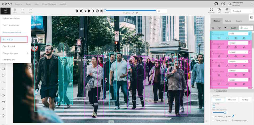
You will see the following dialog:
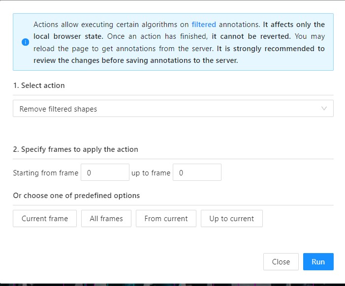
With the following fields:
| Field | Description |
|---|---|
| Select action | Drop-down list with available actions: Note: only Propagate shapes and Remove filtered shapes is available in the community version. |
| Specify frames to run action | Field where you can specify the frame range for the selected action. Enter the starting frame in the Starting from frame: field, and the ending frame in the up to frame field. If nothing is selected here or in Choose one of the predefined options section, the action will be applied to all fields. |
| Choose one of the predefined options | Predefined options to apply to frames. Selection here is mutually exclusive with Specify frames to run action. If nothing is selected here or in Specify frames to run action section, the action will be applied to all fields. |
Convert shapes
Recommended Precautions Before Running Annotation Actions
-
Saving changes: It is recommended to save all changes prior to initiating the annotation action. If unsaved changes are detected, a prompt will advise to save these changes to avoid any potential loss of data.
-
Disable auto-save: Prior to running the annotation action, disabling the auto-save feature is advisable. A notification will suggest this action if auto-save is currently active.
-
Committing changes: Changes applied during the annotation session will not be committed to the server until the saving process is manually initiated. This can be done either by the user or through the auto-save feature, should it be enabled.
To convert shapes, do the following:
-
Annotate your dataset.
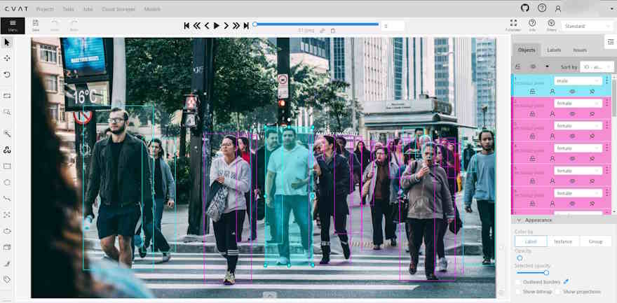
-
Set up filters.
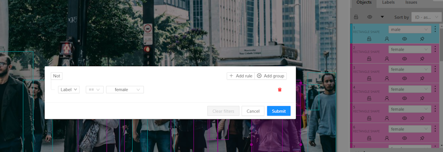
-
From the burger menu, select Run actions.
-
Choose the action you need from the Select action drop-down list.
-
(Optional) In the Starting from frame field, enter the frame number where the action should begin, and in the up to frame field, specify the frame number where the action should end.
-
(Optional) Select an option from Or choose one of the predefined options to apply the action.
-
Click Run.
A progress bar will appear. You may abort the process by clicking Cancel until the process commits modified objects at the end of pipeline.